[1]:
from IPython.display import Image
from IPython.display import Video, HTML, YouTubeVideo
width = 600
Galaxy formation
The formation of galaxies requires understanding the background cosmological model, the initial conditions that led to the seeds of structure, the evolution of perturbations in the Universe, the formation of dark matter halos which then act as the host of a variety of baryonic processes which shape the galaxies. In this chapter, we will go through these basics.
Cosmology
A number of observational results, particularly those from the cosmic microwave background, indicate that we live in an expanding Universe with a simple flat geometry when averaged over large scales, and that the ordinary matter that we are made up of forms a meagre 5 percent of the total energy density budget of the Universe. The rest of it is in the form of dark matter (about 26 percent), and dark energy (about 69 percent). The Universe today also has a tiny amount of its energy density in relativistic species such as photons. Dark matter interacts gravitationally with the ordinary matter, but there is no evidence of dark matter interacting with itself electromagnetically or with the ordinary matter. Dark energy is a mysterious component which causes the accelerated expansion of the Universe.
The expanding Universe model sets the background for structure formation to take place. The expansion of the Universe can be described by a scale factor \(a(t)\) which expresses how physical scales change as a function of time. The physical scales in the expanding Universe can be expressed as
\begin{equation} R_{\rm phys} = R_{\rm com} a(t) \end{equation}
where \(R_{\rm com}\) is called the comoving scale. By convention \(a(t)\) is set equal to unity today. The velocity of objects can then be obtained by differentiating the above equation
\begin{equation} \frac{d}{dt}R_{\rm phys} = \frac{d}{dt} R_{\rm com} a(t) \\ \end{equation}
\begin{equation} \frac{d}{dt}R_{\rm phys} = \dot{a} R_{\rm com} + a(t) \frac{d}{dt} R_{\rm com} \\ \end{equation}
\begin{equation} \frac{d}{dt}R_{\rm phys} = \frac{\dot{a}}{a} R_{\rm phys} + a(t) \frac{d}{dt} R_{\rm com} \end{equation}
The first term which shows that even in the absence of any motion in comoving coordinates, objects separated by distance \(R_{phys}\) will be moving away from each other at velocities proportional to their distances. The proportionality constant is called the Hubble parameter.
Newtonian derivation of the evolution of the scale factor
One can derive the evolution of the scale factor by using Newtonian arguments. Let us assume a uniform density homogenous and isotropic Universe. Consider a shell of mass \(dM\) with radius \(a\) in the Universe. The mass within this shell exerts a gravitational influence on this shell. The equation of motion for this shell will be given by
\begin{eqnarray} \frac{d}{dt} v &=& -\frac{GM}{a^2}\\ v\frac{d}{da} v &=& -\frac{GM}{a^2} \end{eqnarray}
The mass inside the shell will remain the same, as the shells move in and out. Therefore, integrating the above equation we get
\begin{eqnarray} \frac{v^2}{a^2} &=& \frac{8 \pi G \rho }{3} + \frac{C}{a^2}\\ \left(\frac{\dot{a}}{a}\right)^2 &=& \frac{8 \pi G \rho }{3} + \frac{C}{a^2} \end{eqnarray}
This resembles the Friedmann equation that we obtain as solutions to Einstein’s equations for a homogenous and isotropic Universe. The energy density on the right hand side can consist of matter, radiation, dark energy and other terms. Therefore,
\begin{eqnarray} \left(\frac{\dot{a}}{a}\right)^2 &=& \frac{8 \pi G (\rho_\Lambda + \rho_{\gamma} + \rho_{\rm m} )}{3} + \frac{C}{a^2} \end{eqnarray}
The left hand side is nothing but the Hubble parameter. If we can measure it today (the Hubble constant) it can give us a boundary value to solve the above equation and obtain \(a(t)\). If the energy density of the Universe today is equal to the critical density, then the constant \(C\) can be set equal to zero.
\begin{equation} \rho_{\rm crit} = \frac{3H_0^2}{8 \pi G} \end{equation}
The entire equation above can be rewritten as
\begin{eqnarray} \left(\frac{\dot{a}}{a}\right)^2 &=& H_0^2 \left[\frac{(\rho_\Lambda + \rho_{\gamma} + \rho_{\rm m} ) + C'a^{-2}}{\rho_{\rm crit}} \right]\\ \end{eqnarray}
The value of the constant can be determined by working out the above equation at redshift zero. Now let us look at the behaviour of the energy density components. Dark energy behaves in the simplest manner with \(\rho_{\rm \Lambda}=constant\). Non-annihilating and non-interacting dark matter will preserve the number of particles per comoving box, and so the number and hence its mass density will scale as \(a^{-3}\). For radiation, the energy density goes down by \(a^{-4}\). Therefore we have,
\begin{eqnarray} \left(\frac{\dot{a}}{a}\right)^2 &=& H_0^2 \left[\frac{(\rho_\Lambda^0 + \rho_{\gamma}^{0}a^{-4} + \rho_{\rm m}^0 a^{-3} ) + C'a^{-2}}{\rho_{\rm crit}} \right]\\ \left(\frac{\dot{a}}{a}\right)^2 &=& H_0^2 \left[\Omega_\Lambda + \Omega_{\gamma} a^{-4} + \Omega_{\rm m}^0 a^{-3} + \Omega_{\rm k}^0 a^{-2} \right]\\ \end{eqnarray}
where \(\Omega_{\rm k}^0 = (1-\Omega_{\Lambda}-\Omega_{\rm m} - \Omega_{\gamma})\). This equation can then be solved to obtain the evolution equation for \(a(t)\). Depending upon the energy density content of the Universe, one can have solutions where \(a(t)\) continues to increase at an ever decreasing rate, or \(a(t)\) increases, reaches a maximum size, and then starts to decrease, or \(a(t)\) eventually start to increase exponentially.
Solve the Friedmann equation for the matter only case, where \(\Omega_{\rm m}=1\) and the rest of the energy components are equal to zero.
Given that the energy density of radiation today is about \(10^{-4}\). Can you compute the scale factor where the energy density in radiation and matter were equal.
Given the current cosmological parameters constrained by Planck, compute the scale factor where the energy density in dark energy and matter were equal.
Solve the Friedmann equation for the current cosmological parameters as constrained by the Planck collaboration.
The inhomogeneous Universe
At the very early stages the Universe also underwent an exponential expansion called inflation. You will learn about it in the cosmology course. Tiny quantum fluctuations during the inflationary era get stretched to astronomical scales, and these fluctuations act as the seeds for the formation of structure in the Universe. The fluctuations are Gaussian in nature. Let us try to understand the statistical properties of these fluctuations.
The overdensity, \(\delta(\vec{x})\) is given by
\begin{equation} \delta(\vec{x}) = \frac{\rho(\vec{x})}{\bar\rho} - 1 \end{equation}
Given that the fluctuations are Gaussian one can characterize them fully, by the mean (zero by construction), and the covariance \(\langle\delta(\vec{x})\delta(\vec{x}+\vec{r}) \rangle\). Invoking translational and rotational invariance, this quantity should only depend upon the modulus of the distance \(|\vec{r}|\). This quantity is called the two point correlation function, \(\xi(r)\).
It is often useful to work in Fourier space. The overdensity field in Fourier space is given by
\begin{equation} \delta(\vec{k}) = \int d^3{\vec x} \,\delta(\vec{x}) \,e^{-i\vec{k}.\vec{x}} \end{equation}
The correlation in Fourier space, \(\langle \delta(\vec{k})\delta(\vec{k'}) \rangle\) is then given by
\begin{eqnarray} \langle \delta(\vec{k})\delta(\vec{k'}) \rangle &=& \int d^3 \vec{x'} \int d^{3} \vec{x} \langle \delta(\vec{x}) \delta(\vec{x}') \rangle e^{i(\vec{k}.\vec{x}+\vec{k}'.\vec{x}')} \\ &=& \int d^3 \vec{x'} \int d^{3} \vec{y} \,\xi(\vec{y}) e^{i\vec{k}.\vec{y}}e^{i(\vec{k}+\vec{k'}).\vec{x'}}\\ &=& (2\pi)^3 P(\vec{k}) \delta_{\rm D} (\vec{k}+\vec{k'}) \end{eqnarray}
where the power spectrum \(P(\vec{k})\) is the fourier transform of the correlation function \(\xi(\vec{r})\). Rotational invariance further demands that the power spectrum should only be a function of the modulus of \(\vec{k}\). The Power spectrum has dimensions of volume, so the dimensionless quantity \(\Delta(k)\) can be constructed which represents the power per logarithmic interval in \(k\),
\begin{equation} \Delta(k) = \frac{k^3}{2\pi^2} P(k) \end{equation}
Similar to the density fluctuations one can also consider potential fluctuations and the power spectrum of potential fluctuations. The potential fluctuations are related to the density fluctuations with the Poisson equation,
\begin{eqnarray} \nabla^2 \delta_{\rm \phi} \propto \delta \\ k^2 \delta_{\rm \phi}(k) \propto \delta(k) \end{eqnarray}
The power in the initial potential fluctuations per logarithmic interval of \(k\) set by inflation is constant due to scale invariance (see cosmology lectures this semester). This implies that the initial density power spectrum
\begin{equation} P(k) \propto k \end{equation}
The index in the power spectrum has been measured by data, and is quite close to unity although not exactly unity. Since inflation ends at a certain epoch, inflation in fact predicts a slope close to unity, but with slight deviations. This deviation has now been measured at more than 5\(\sigma\) in the data.
These fluctuations are set at the end of inflation. The Universe then enters an era of radiation domination. The density fluctuations set at the end of inflation will grow. There are two regimes to consider, one for fluctuations whose wavelengths are beyond the horizon, and the others where the wavelength is within the horizon. The growth of fluctuations which are larger than the horizon can be understood by understanding that such fluctuations behave as if they are in a Universe of their own, but with a different curvature. If the background cosmology is flat, then the background Universe obeys
\begin{equation} \left(\frac{\dot{a}}{a}\right)^2 = \frac{8\pi G \rho}{3} \end{equation}
while the Universe with the fluctuation will have
\begin{equation} \left(\frac{\dot{a_1}}{a_1}\right)^2 = \frac{8\pi G \rho(1+\delta)}{3} + \frac{C'}{a_1^2} \end{equation}
As the fluctuations are small, the differences between \(a_1\) and \(a\) are bound to be small. This implies that the two scale factors closely follow each other when the fluctuations are small. Then we can write,
\begin{eqnarray} \frac{8\pi G \rho(1+\delta)}{3} + \frac{C'}{a_1^2} = \frac{8\pi G \rho}{3} \end{eqnarray}
which allows us to show that
\begin{eqnarray} \delta \propto \frac{1}{a^2\rho} \end{eqnarray}
In the radiation dominated era, \(\rho \propto a^{-4}\), thus the fluctuations beyond the horizon grow with the scale factor \(a^2\), while in the matter dominated era where \(\rho \propto a^{-3}\), the fluctuation grow as the scale factor.
For the growth of fluctuations with wavelengths within the horizon, one needs to consider the timescales for collapse of these perturbations to the time scale of expansion. The time scale for collapse is given by \((G\rho_{\rm m})^{-1/2}\) while the time scale for expansion is given by \((G\rho_{\rm tot})^{-1/2}\). In the radiation dominated era, the modes within the horizon cannot grow as the expansion time scale is shorter than the collapse time scale. In the matter dominated era the time scales are comparable and the fluctuations are able to grow.
This results in a characteristic power spectrum which has a turnover imprinted at the scale of matter radiation equality. This scale has also been seen in observations now.
Halo formation
The equations for the growth of perturbations in the linear regime and the collapse of spherical top hat perturbation will be discussed in the cosmology class. There are two important learnings that we will borrow from the cosmology class. In the linear regime in the matter dominated era, fluctuations grow with a rate which is independent of the wavenumber \(k\). Spherical halos form when the linearly extrapolated density field reaches a critical threshold value of \(\delta_{\rm c}\).
Thus dark matter halos form at the density peaks in the initial density field. The abundance of these halos as a function of mass is given by the frequency of occurence of such peaks. The bigger the size of the density fluctuation which reaches this critical threshold, the larger the mass.
To get the abundance of halos as a function of mass \(M\), consider a sphere of radius \(R\), where
\begin{equation} M = \frac{4}{3} \pi R^3 \bar \rho \end{equation}
We can compute the variance of the density field when averaged over a sphere of radius \(R\), by considering the field \(\delta_{R}(\vec{x})\) which smooths the overdensity field with a kernel \(W\) with radius \(R\). Thus
\begin{equation} \delta_{R}(\vec{x}) = \int d^3 \vec{x'} \delta(\vec{x}') W_R(\vec{x}-\vec{x}') \end{equation}
Here the window function \(W_R\) is defined such that
\begin{equation} W_R(\vec{r}) = 0 \,\, \forall |\vec{r}|\gt R \end{equation} \begin{equation} W_R(\vec{r}) = \frac{3}{4\pi R^3} \,\, \forall |\vec{r}| \leq R \end{equation}
The variance of this field is then given by
\begin{eqnarray} \langle \delta_R(\vec{x})^2 \rangle &=& \int d^3 \vec{x'} \int d^3 \vec{x''} \langle \delta(\vec{x}')\delta(\vec{x}'')\rangle W_R(\vec{x}-\vec{x}') W_R(\vec{x}-\vec{x}'') \\ &=& \int d^3 \vec{x'} \int d^3 \vec{x''} \xi(\vec{x}'-\vec{x}'') W_R(\vec{x}-\vec{x}') W_R(\vec{x}-\vec{x}'') \end{eqnarray}
This double convolution can be easily evaluated in Fourier space and then transformed back to obtain
\begin{eqnarray} \sigma_{R}^2 = \langle \delta_R(\vec{x})^2 \rangle &=& {\rm FT} \left[ P(k) W_R(k)^2 \right] \end{eqnarray}
As \(R\rightarrow \infty\), the variance goes to zero, but its behaviour with \(R\) will depend upon the power spectrum. For the power spectrum in the concordance cosmological model, the power spectrum just decreases with \(R\). Now the initial conditions could be evolved with the linear growth rate, and could be smoothed with a large radius \(R\) and ask if there is any point which has a density above the critical density at a given redshift. The radius can be shrunk until there are points which have \(\delta_R(\vec{x})\) greater than the critical density threshold. Those locations will correspond to the particles in the initial density field which lead to the formation of a halo of mass \(M\). Continuing the march downwards would allow us to identify the halos starting from initial conditions.
The fraction of mass bound in halos of mass \(M\) and above can then be calculated as
\begin{equation} F(>M) = \int_{\delta_c}^{\infty} P(\delta|\sigma_{\rm R}) \end{equation} \begin{equation} F(>M) = \frac{1}{2}{\rm erfc} \left(\frac{\delta_c}{\sqrt{2}\sigma_{\rm R}}\right) \end{equation}
The number density of halos with mass in the range \([M, M+dM]\) is given by
\begin{equation} \frac{d}{dM} n(>M) = \frac{\bar\rho}{M}\frac{d}{dM}F(>M) \end{equation} \begin{equation} \frac{d}{dM} n(>M) \propto \frac{\bar\rho}{M^2} \exp\left(-\frac{\delta_{\rm c}^2}{2\sigma^2}\right)\frac{\delta_c}{\sigma}\frac{d\ln\sigma}{d\ln M} \end{equation} This particular way to derive the halo mass function was first presented by Press and Schechter in 1974. The mass function they found showed that only half of the mass in the Universe would be bound in halos. So they had added a fudge factor of 2 to the mass function they obtained with these arguments. The factor of 2 is already missing in the first equation of the above argument. This was pointed out by Bond et al. 1992. The solution for the statistical problem corresponding to this problem was first presented by Chandrasekhar some time before (he was not solving the mass function problem). It has to do with regions which are underdense than the critical threshold but are part of bigger overdensities (it is called the cloud-in-cloud problem).
The Press Schechter mass function qualitatively reproduces the halo mass function observed in simulations, you see a power law at the low mass end, and an exponential drop off at the massive end. There have been many advances in understanding the halo mass function theoretically with more quantitative success: in particular the use of ellipsoidal collapse rather than spherical collapse to set the critical threshold for collapse (e.g., Sheth, Mo, Tormen 1999, 2001), stochasticity in the critical threshold (e.g., Corasaniti et al 2011), statistics of peaks (Paranjape et al. 2013). However, these approaches often lead to better functional forms whose free parameters are tuned in order to fit the halo mass function in arbitrary cosmologies.
The mass function appears fairly universal, but there are small deviations and these have been now well characterized with the help of numerical simulations. Fitting functions or interpolation routines that can compute the mass function for a given mass and redshift are available. The following figure from Tinker et al. (2008) shows a comparison between the halo mass function as measured from numerical simulations and the Press Schechter mass function.
[2]:
Image("images/mass_function.png", width=width)
[2]:
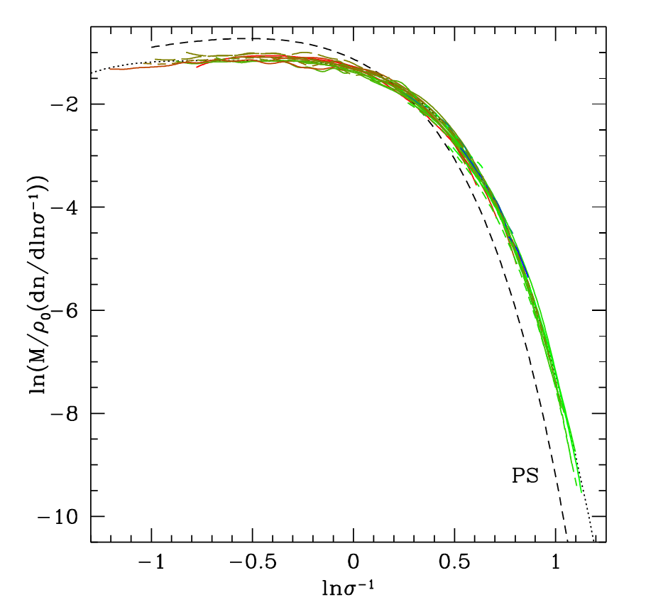
A technical caveat while interpreting some of these plots: when halos are identified in simulations they are assigned boundaries. These boundaries define a halo to be a certain factor (200, 500, 2500 are common choices) overdense compared to a reference density (the mean matter density or the critical density are the common choices). The measured mass functions can differ depending upon these choices. There is ongoing research in order to identify if there are halo definitions which give mass functions similar to that predicted by Press Schechter formalism.
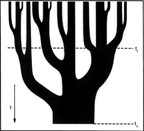
Halo finding algorithms are run for snapshots of simulations taken at different times. The halos identified in this manner can be connected through a progenitor-descendant relationship which can be depicted as a merger tree (e.g. see Behroozi et al. 2012).
[3]:
Image(url="https://ned.ipac.caltech.edu/level5/March12/Silk/Figures/figure10.jpg", width=width)
[3]:
Galaxy formation
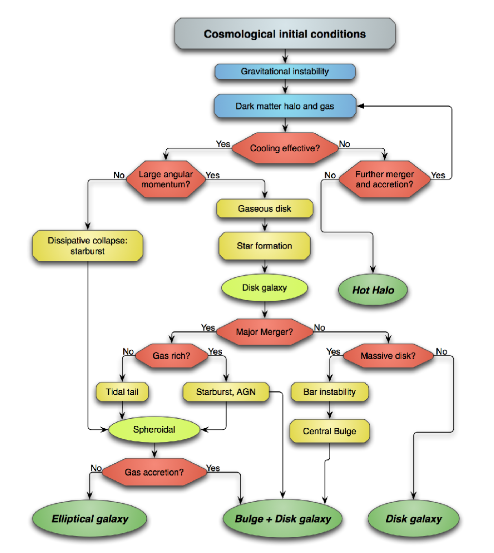
Galaxy formation then takes place in these haloes through a variety of processes. A flow-chart for the formation of galaxies can be found in the image below which is adapted from Mo, van den Bosch & White (2010) by Niemi (2011). The flow chart shows the various processes that lead to the formation of galaxies. The diverse paths setup by the cosmological initial conditions lead to diverse outcomes, and therefore the diversity of the galaxy population.
[4]:
Image("images/galform.png", width=width)
[4]:
Coding project
Although we will deal with some of this complexity in our course, we will follow a simpler phenomenological approach for our coding project. We will follow the simple galaxy stellar mass evolution of Becker 2015. In this model we will use merger trees from numerical simulations in order to obtain the growth and the merger history of dark matter halos. Each student will receive a set of merger trees to work on. The merger trees will be marked with a descendant at \(a=1\), and then specify a set of progenitors at every snapshot step with \(a<1\).
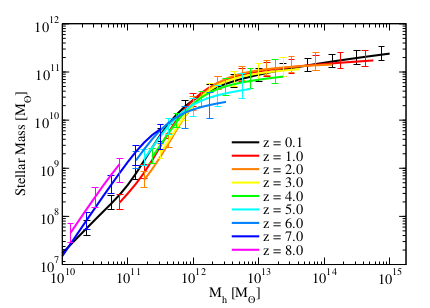
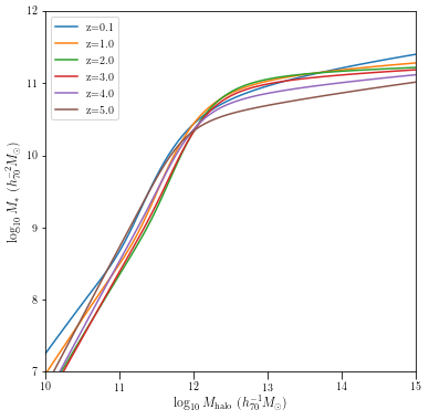
The stellar mass halo mass relation has been constrained over a large range of redshifts by Behroozi et al. 2013 using a variety of observations including stellar mass functions, star formation histories, etc. Here are the results.
[5]:
Image("images/behroozi.png", width=width)
[5]:
For a given tree, we will start with high redshift progenitors (choose a snapshot close to redshift 5). We will populate them with galaxies with stellar masses that follow the above relation at redshift 5.
[6]:
from IPython.display import Image
from IPython.display import Video, HTML, YouTubeVideo

import pylab as pl
%pylab inline
conf = %config InlineBackend.rc
conf["figure.figsize"] = (6, 6)
conf['savefig.dpi']=100
conf['font.serif'] = "Computer Modern"
conf['font.sans-serif'] = "Computer Modern"
conf['text.usetex']=True

width = 600
%config InlineBackend.rc
%pylab inline
Populating the interactive namespace from numpy and matplotlib
Populating the interactive namespace from numpy and matplotlib
[7]:
import numpy as np

class Behroozi_2013a:
    def __init__(self):
        self.eps0=-1.777;
        self.epsa=-0.006;
        self.epsz=-0.000;
        self.epsa2=-0.119;

        self.xM10=11.514;
        self.xM1a=-1.793;
        self.xM1z=-0.251;

        self.alp0=1.412;
        self.alpa=-0.731;

        self.delta0=3.508;
        self.deltaa=2.608;
        self.deltaz=-0.043;

        self.gamma0=0.316;
        self.gammaa=1.319;
        self.gammaz=0.279;


    def evolved_factors(self,zz):
        a=1./(1.+zz);
        nu=np.exp(-4*a*a);
        alp=self.alp0+self.alpa*(a-1.0)*nu;
        delta=self.delta0+(self.deltaa*(a-1.)+self.deltaz*zz)*nu;
        gamma=self.gamma0+(self.gammaa*(a-1.)+self.gammaz*zz)*nu;
        eps=self.eps0+(self.epsa*(a-1.0)+self.epsz*zz)*nu+self.epsa2*(a-1.)
        xM1=self.xM10+(self.xM1a*(a-1.0)+self.xM1z*zz)*nu;
        return nu, alp, delta, gamma, eps, xM1

    def fbeh12(self, x, nu, alp, delta, gamma):
        return -np.log10(10.**(-alp*x)+1)+delta*(np.log10(1.+np.exp(x)))**gamma/( 1. + np.exp(10.**-x) )

    def SHMRbeh(self, xmh,zz):
        nu, alp, delta, gamma, eps, xM1 = self.evolved_factors(zz)
        xmstel=eps+xM1+self.fbeh12(xmh-xM1, nu, alp, delta, gamma)-self.fbeh12(0.0, nu, alp, delta, gamma);
        return xmstel;

aa = Behroozi_2013a()
Mhalo = np.linspace(9.0, 15.0, 100)

ax = pl.subplot(111)
for zz in [0.1, 1.0, 2.0, 3.0, 4.0, 5.0]:
    Mstel = aa.SHMRbeh(Mhalo, zz)
    ax.plot(Mhalo, Mstel, label="z=%.1f" % zz)

ax.set_xlim(10.0, 15.0)
ax.set_ylim(7.0, 12.0)
ax.set_xlabel(r"$\log_{10} M_{\rm halo}$ ($h_{70}^{-1}M_\odot$)")
ax.set_ylabel(r"$\log_{10} M_*$ ($h_{70}^{-2}M_\odot$)")
pl.legend()
/usr/lib/python3.7/site-packages/ipykernel_launcher.py:37: RuntimeWarning: overflow encountered in exp
[7]:
<matplotlib.legend.Legend at 0x7f9f2712ea10>
findfont: Font family ['serif'] not found. Falling back to DejaVu Sans.
Once populated, we would like to track the growth of stellar mass in these halos through the merger trees. If we assume that all halos have their cosmological fraction of baryons \(f_{\rm b} = \Omega_{\rm b}/{\Omega_{\rm m}}\) within them, then the halo merger trees can tell us about the availability of new gas within halos. This will just be given by \(\Delta M_{\rm gas} = \Delta M_{\rm halo} \times f_{\rm b}\). The conversion of this gas into stellar mass can be obtained by following the simple equation
\begin{equation} \frac{dM_{*}}{dt} = f_{\rm b}\frac{dM_{\rm halo}}{dt} \times {\rm SFE}(M_{\rm halo}, z) \end{equation}
We will use the instantaneous star formation efficiencies of halos as constrained by Behroozi et al. (2013b).
[8]:
Image("images/behroozi_sfe.png", width=width)
[8]:
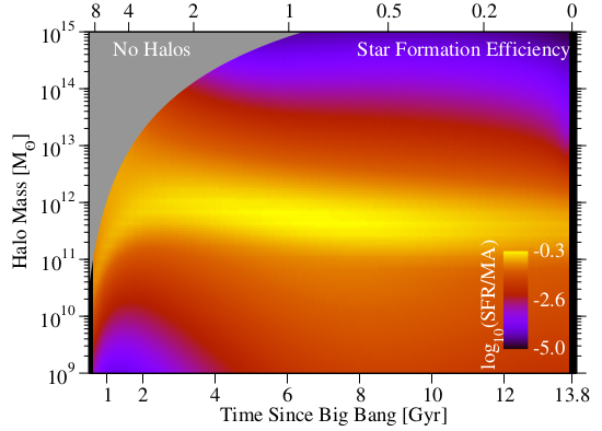
The above plot is quite striking. Star formation is most efficient in halos of mass \(10^{12}M_{\odot}\) and falls off on either side of this mass scale. We will use this data in our equation for stellar mass growth. The data for the above plot can be downloaded from the following link.
Becker et al. (2015) starts with these assumptions and follows the growth of stellar mass in the main galaxy as well as in a component called the intracluster light. Intracluster light is supposed to be the light from stars of shredded satellite galaxies. These are prominently seen as the faint fuzzy glow in cluster scale halos in observations (see an example from the Hubble Space Telescope below).
[9]:
Image(url="https://media.stsci.edu/uploads/image/display_image/4024/STSCI-H-p1720a-d-1280x720.png", width=width)
[9]:

Becker et al (2015) come up with the following rules to evolve galaxies in the merger tree. In the halo merger tree, a given descendant halo may have either one, two or many progenitors. In case it has just one progenitor, the descendant halo will get the stellar mass of its progenitor, and any mass of stars the progenitor will form based on the star formation efficiency. The intracluster light like component just gets passed over as is from the progenitor to the descendant. In case of a binary merger, the stellar mass of the progenitors along with any newly formed stars will be passed to the stellar mass component of the descendant, and the ICL component gets passed along from both the progenitors. In case of a multiple galaxy merger, only the central stellar mass component of the most massive progenitor and any newly formed stellar mass is passed to the descendant. The rest of the stellar mass (both central and ICL component) in all the other progenitors is added to the ICL like component of the progenitor and assigned as the ICL component of the descendant.
Once these rules are coded up, we can track the growth of stellar mass of galaxies with time and compare to the observationally measured evolution of stellar mass functions. That will be the main scientific goal of the project.