Observations of galaxies
In this chapter, we will walk through some of the basics of astronomical observations of galaxies.
[1]:
from IPython.display import Image
from IPython.display import Video, HTML, YouTubeVideo
import numpy as np
import pylab as pl
%pylab inline
conf = %config InlineBackend.rc
conf["figure.figsize"] = (6, 6)
conf['savefig.dpi']=100
conf['font.serif'] = "Computer Modern"
conf['font.sans-serif'] = "Computer Modern"
conf['text.usetex']=True

width = 600
%config InlineBackend.rc
%pylab inline
Populating the interactive namespace from numpy and matplotlib
Populating the interactive namespace from numpy and matplotlib
Measuring light from galaxies
The bolometric luminosity of a galaxy tells us the total energy per unit time emitted by the components of a galaxy. The luminosities of galaxies are often measured in specific wavelength bands. This is achieved by passing the light coming into the telescope via a filter system like the one shown below.
[2]:
Image(url="http://www.astro.uvic.ca/~gwyn/cfhtls/photz/cfhtlsugriz.gif")
[2]:

This shows the filter response curves for the Canada France Hawaii Telescope Legacy Survey (CFHTLS). The light colored lines show the light which gets transmitted by the actual filter on the telescope. This then has to be further multiplied by losses due to the telescope (mirror, optics), and the CCD quantum efficiency. This results in the final filter response curves seen in bold.
The telescope measures the surface brightness of objects (energy per unit time per unit area per solid angle) that arrives at the telescope. The surface brightness when integrated over the solid angle covered by the galaxy gives its flux (energy per unit time per unit area). The flux is related to the luminosity by \begin{equation} F = \frac{L}{4\pi D_{\rm l}^2} \end{equation} where \(D_{\rm l}\) is the luminosity distance to the galaxy.
The observed flux from a galaxy, \(\tilde{f}\), in a given band, is related to its intrinsic spectral energy distribution, \(f(\lambda)\), by \begin{equation} \tilde{f} = \int f_{\lambda} R(\lambda) A(\lambda) G(\lambda) d\lambda \end{equation} where \(R(\lambda)\) is the total filter response functions shown above, \(A(\lambda)\) is the atmospheric extinction due to the light traveling at a given angle in the atmosphere, \(G(\lambda)\) is the extinction due to dust in the Milky Way towards the direction of the galaxy. The atmospheric and galactic extinction are corrected for using airmass and extinction corrections.
How would one determine the dependence of the atmospheric extinction on the elevation of an object?
Click for Answer
Answer could be potentially written here.
Astronomers use the logarithmic scale of apparent magnitudes to describe fluxes. A difference of 5 magnitudes corresponds to a difference of 100 in flux. Thus two objects with magnitude \(m_1\) and \(m_2\) are related by \begin{equation} m_1 - m_2 = -2.5 \log_{10}{\frac{f_1}{f_2}} \end{equation}
This defines the magnitude scale upto a constant. The constant was typically chosen such that the star Vega corresponds to magnitude zero. These are called Vega magnitudes. However the system was standardized to remove the necessity of a reference by defining
\begin{equation} m = -2.5 \log_{10}{f} - 48.60 \end{equation} where \(f\) is in units of \({\rm erg\,s}^{-1}{\rm cm}^{-2}{\rm Hz}^{-1}\).
The flux of an object is dependent upon its distance from us. Thus to get a measure of the luminosity of a galaxy independent of the distance, astronomers define absolute magnitude, as the magnitude that the object would have if it was at a distance of 10 parsec. The absolute magnitude can be calculated from the apparent magnitude only if its luminosity distance is known.
\begin{equation} m - M = 5 \log_{10} \frac{d_{\rm L}}{10 \,{\rm pc}} = 5 \log_{10} \frac{d_{\rm L}}{{\rm Mpc}} + 25.0 \end{equation}
One can also use the above equation to obtain the distance if the absolute magnitude of the object is known based on some theoretical or empirical grounds.
Suppose I know that supernovae of a particular type all have the same luminosity, what can we infer from the apparent magnitudes of two supernovae?
Click for Answer
Answer could be potentially written here.
Spectroscopy of galaxies
The light passed through a spectroscopic instrument disperses the flux as a function of wavelength. The quantity \(f_{\lambda} d\lambda\) denotes the flux obtained within a wavelength range \(\lambda\pm d\lambda/2\). The light is gathered from a slit or a fiber and sent towards the spectroscopic instrument. Large surveys can be carried out if the telescope has a multi-object or multi-fiber spectroscopic capability, which can take light from multiple targets in the field of view of the telescope. Nearby galaxies can also be targeted using integral field spectroscopy where multiple fiber bundles are put together to get the spectrum in different regions of the galaxy.
The spectroscopic studies of galaxies reveal continuum emission which is punctuated at different places by emission and absorption lines. Absorption and emission lines reveal the composition and ionization state of the stellar atmospheres and the gas within the galaxy.
Spectra are also a crucial input to the study of galactic dynamics. The photons arriving from the galaxy towards us are shifted in wavelength due to the motion of the emitters or absorbers. This shift in wavelength is a combination of the cosmological expansion as well as the motion within the galaxy. Although all the photons will share the cosmological redshift, the random motions within the galaxy blur out the lines due to the velocity distribution. The location of the line thus contains information about the streaming motion while the shape of the line thus contains information about the velocity distribution.
Spectra of different type of galaxies
The spectra of galaxies can show different spectrum dependent upon their type. Here are some examples:
[3]:
Image(url="http://astroweb.cwru.edu/cassie/323/jan22p9.jpg")
[3]:
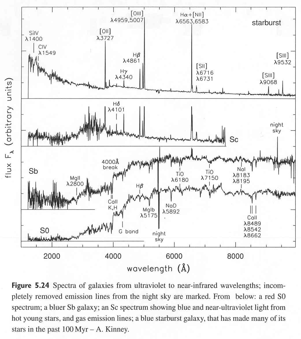
Star forming galaxies show many distinct emission lines along with a broad blue continuum emission. The equivalent width of these emission lines decreases as we move to objects with bigger and more prominent bulges such as the S0s. The continuum emission from S0s is also lacking output in blue which gives them a redder appearance.
Can you think of how the broad band continuum features could be used to obtain a redshift using just the photometry of galaxies?
Elliptical galaxies
Structure of elliptical galaxies
The surface brightness profiles of elliptical galaxies can be well fit by the profile introduced by Sersic in 1963 (Caon et al. 1990, 1993, 1994).
\begin{equation} I(R) = I_{\rm e} {\rm exp}\left( -b_n \left[ \left( \frac{R}{R_{\rm e}} \right)^{1/n} - 1 \right] \right) \end{equation}
The Sersic profile has three free parameters, \(I_{\rm e}, R_{\rm e}\) and \(n\). The term \(b_n\) is used to set the normalization of the profile such that the integrated light within the effective radius \(R_{\rm e}\) is equal to half of the total light from the galaxy.
Compute the relation between central surface brightness (\(\mu_0=-2.5\log_{10} I_0\)) and the effective surface brightness (\(\mu_e=-2.5\log_{10} I_e\)).
Compute difference between effective surface brightness and the mean effective surface brightness averaged over all radii.
What value of \(n\) for the Sersic profile gives rise to an exponential profile?
Prugniel and Simien (1997) also gave approximate expressions for the three dimensional density profile which when projected gives rise to the Sersic profile.
Click for Answer
Answer could be potentially written here.
[4]:
class sersic:
    def __init__(self, Ie, Re, n):
        self.Ie = Ie
        self.Re = Re
        self.n = n
        if self.n>=0.5 or self.n<=10:
            self.bn = 1.9992 * n - 0.3271
        else:
            print ("Use n between 0.5 and 10 for approximation to work")
            print ("General purpose n is left as exercise, see below and contribute code")

    def profile(self, R):
        facR = (R/self.Re)**(1/self.n) - 1
        expfac = -facR*self.bn
        return -2.5*np.log10(self.Ie*np.exp(expfac))


ax = pl.subplot(111)
#R = np.logspace(-3, 1.6, 100)
R = np.linspace(0, 30.0, 100)
#ax.set_xscale("log")
#ax.set_yscale("log")
ax.set_ylim(29.0, 18.0)
ax.set_xlim(0.0, 30.0)


Ie = 10**(-25.0/2.5)
Re = 10.0

for nn in [0.5, 1.0, 2.0, 4.0, 10.0]:
    aa = sersic (Ie, 10.0, nn)
    ax.plot(R, aa.profile(R), label="n=%.1f" % nn)
ax.legend()

ax.axhline(25.0, alpha=0.1)
ax.axvline(10.0, alpha=0.1)
ax.set_xlabel("R")
ax.set_ylabel(r"$\mu$")
[4]:
Text(0, 0.5, '$\\mu$')
findfont: Font family ['serif'] not found. Falling back to DejaVu Sans.
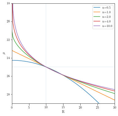
The Sersic profile is an empirical profile. Higher concentration of light towards the centers correspond to larger values of n. Elliptical galaxies, despite their varied formation history, all seem to settle down in this particular profile. Here are a couple of examples from Caon et al. (1993), NGC 4552 with n=13.9 and NGC 4464 with n=2.4.
[5]:
Image("images/Caon1993.png", width=width)
[5]:
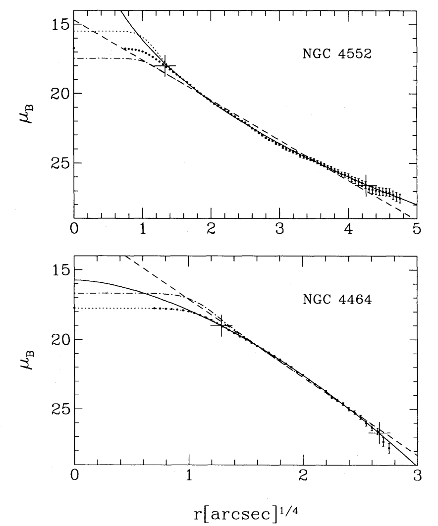
Notice the flattening towards the innermost regions. Part of it could be physical while part of it due to the point spread function. The situation improved after the Hubble Space telescope was launched. Here are a couple of interesting examples from the HST (Graham et al. 2003), one showing a deficit, the other one being well fit by the Sersic profile.
[6]:
Image("images/Graham2003.png", width=width)
[6]:
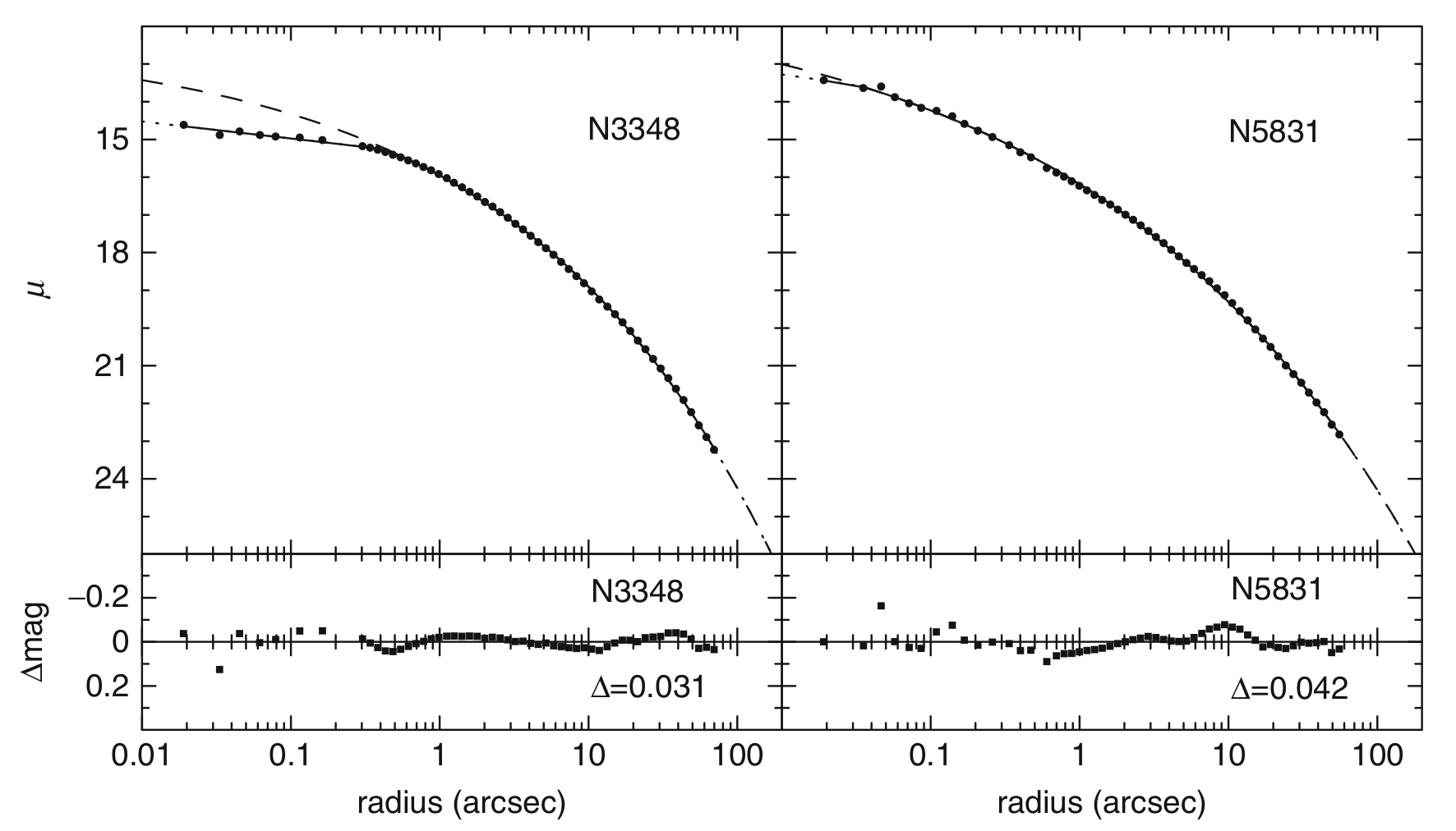
There is quite an extensive literature about whether the inner regions show a cored structure and what empirical profile can be used to describe those. The Nuker law, core-Sersic profile are some of the empirical functions used to describe this behaviour in the inner regions.
What could cause some galaxies to have cores? The centers of elliptical galaxies are supposed to be sites of super massive binary black hole coalescences. During this coalescence, the stars in the inner regions can get kicked out due to 3 body interactions. This could result in a deficit of light at the center. You need a few massive major mergers in order to create a core, and depending upon the evolution history of a galaxy, it could indeed undergo a few such major mergers. Brighter ellipticals typically have such cores.
Fainter galaxies on the other hand can have excess light near the centers compared to the Sersic profile. These are due to nuclear star clusters. Such excess light can often be fit as a Gaussian component (e.g., Wadadekar et al. 1999) or a point source component in addition to the Sersic profile.
In addition to the deviations from Sersic in the innermost regions, the light profiles in the outskirts of Brightest cluster galaxies (BCGs) can show excess light compared to the Sersic fit in the inner regions. This is due to the presence of intracluster light. Although it is difficult to understand where the actuall stellar mass of the BCG ends and the intracluster light begins, there are some indications based on the 2-d profile fits that there is a change in the ellipticity profiles (Gonzalez et al. 2005). One has to be very careful about background subtraction issues when dealing with intracluster light. If the background is estimated locally in a small enough patch then the intracluster light could just get subtracted from the outskirts of galaxies.
The two dimensional shapes of ellipticals
The isophotal shapes of elliptical galaxies can be commonly fit with ellipses, with the minor-to-major axis ratios (b/a) and the angle of the major axis with respect to a fixed reference direction in the plane of the sky. The ellipticity can be different at different distances of isophotes from the center, there could be twists in the isophotes as well.
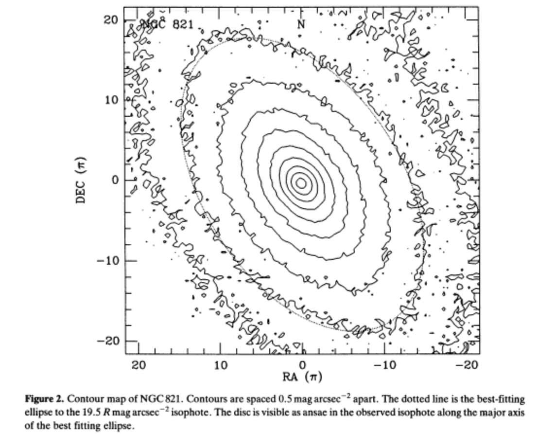
However, there are small deviations seen in the isophotes from ellipses. See for example the following examples from Lauer (1985).
[7]:
Image("images/disky_elliptical.png", width=width)
[7]:
[8]:
Image("images/boxy_elliptical.png", width=width)
[8]:
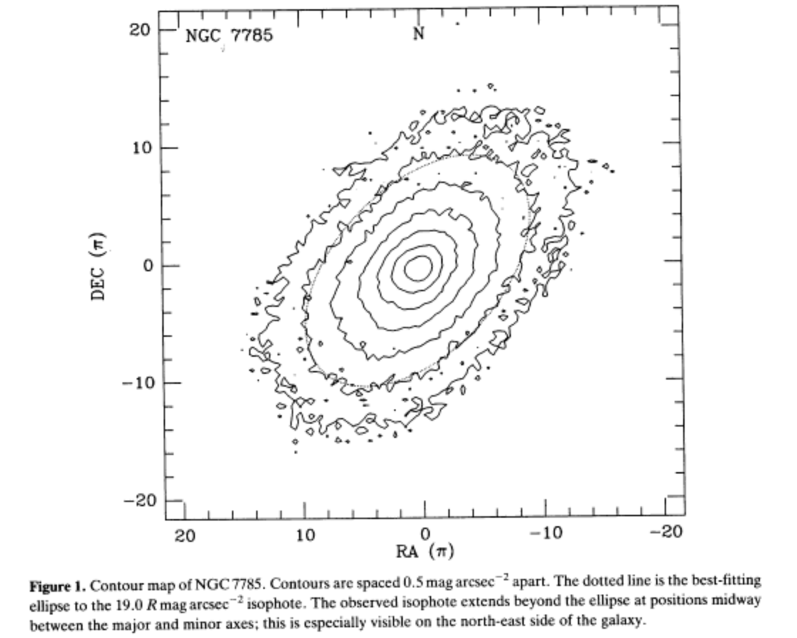
These deviations can be characterized by Fourier coefficients.
\begin{equation} \Delta \phi = R_{\rm iso}(\phi) - R_{\rm ell}(\phi) = a_0 + \sum_{n} \left[a_n cos(n\phi) + b_n sin(n\phi)\right] \end{equation}
The value of \(R_{\rm ell}(\phi)\) is obtained by varying a_0, a_1, b_1, a_2, b_2. The value of odd \(n\) will give deviations from axisymmetry. The sign of \(a_4\) in particular tells about diskiness (\(a_4 \gt 0\)) or boxiness (\(a_4 \lt 0\)) of the isophotes.
Alternative ways to quantify deviations from elliptical isophotes is by looking at the variation of surface brightness along the best fit elliptical isophote.
Empirically, there are correlations between disky or boxy ellipticals and other properties of elliptical galaxies. Boxy ellipticals are brighter, with significant dispersion compared to rotation, larger radio and X-ray emission. Disky ellipticals are fainter, have significant rotation, and less radio or Xray emission.
Structural scaling relations
The concentration of elliptical galaxies (i.e. the Sersic index) is correlated with the luminosity/stellar mass and the central surface brightness in a linear fashion (see e.g. compilation by Graham and Guzman 2003).
[9]:
Image("images/ellipticalsSR.png", width=width)
[9]:
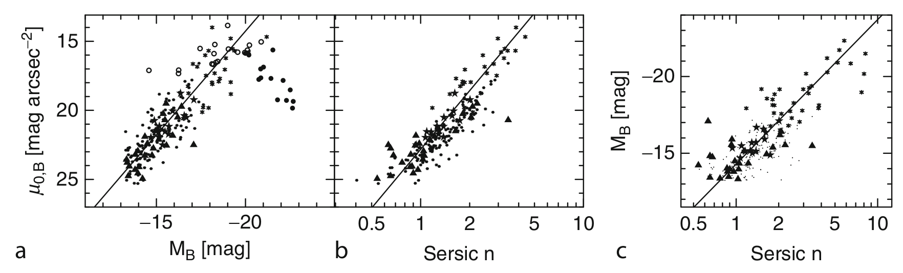
The central surface brightness scales linearly with the magnitude of the ellipticals for galaxies fainter than \(M_B>-20.0\). The dropoff for the brightest galaxies is related to the central deficit of light in the brighter galaxies. The central surface brightness assuming a direct extrapolation of the Sersic profile towards the centers of such galaxies does lie on the linear relation.
Removing those galaxies (since the Sersic profile fit is not great), the central surface brightness scales with the sersic index - brighter central surface brightness galaxies have more concentrated profiles. These two scaling relations imply brighter ellipticals have more concentrated profiles.
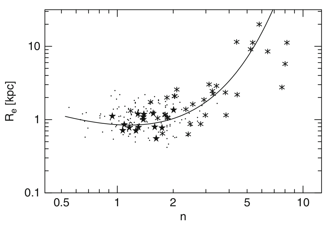
The above scaling relations can then be converted to relations between luminosity and effective surface brightness of galaxies, the luminosity-size relation, the size concentration relation, the size effective brightness relations. From the compilations in Graham 2013, these relations look non-linear (curved), but can be explained by the above linear relations and thus can explain the dichotomy seen in the non-linear relations between dwarf elliptical galaxies (\(M_B \gt -18.0\)), and normal/luminous elliptical galaxies \(M_B \lt -18.0\) in a simple manner.
[10]:
Image("images/ellipticalsSRb.png", width=width)
[10]:
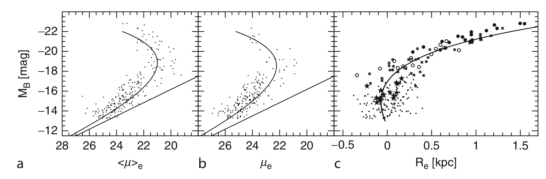
[11]:
Image("images/ellipticalsSRc.png", width=0.5*width)
[11]:
Colors of elliptical galaxies
Elliptical galaxies have a red color because of the 4000A break straddling broad band filters. At same redshift, brighter ellipticals typically have redder color with color proportional to the magnitude (see figure below of members of the nearby Coma cluster of galaxies from Bower et al. 1999). The tightness of this relation in color can constrain the star formation history of the galaxy. The tightness of the color magnitude relation of ellipticals is useful to identify galaxy clusters in imaging surveys.
Typically most of the stars that have been assembled in an elliptical form at very early times, although a number of them may have been formed in some other systems and then accreted on to the current elliptical via mergers. Mergers also reveal that the outskirts of elliptical galaxies are bluer compared to the innermost regions.
[12]:
Image(url="https://ned.ipac.caltech.edu/level5/March06/Renzini/Figures/fig3.jpg", width=width)
[12]:

Kinematic scaling relations
The rotation velocities seen within ellipticals are quite small, especially at the bright end. A quantitative measure of the rotation is the ratio of maximum line-of-sight velocity difference from the average velocity (due to redshift for further away galaxies) to the line of sight velocity dispersion. If the elliptical galaxy is flattened by rotation one can expect that the ellipticity of the galaxy is related to this ratio. Larger the ellipticity (1-b/a), larger the rotation. Here is a compilation of data from the Mo, van den Bosch and White textbook.
[13]:
Image("images/vbysigma.png", width=width)
[13]:
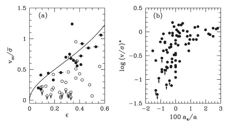
The open circles are brighter ellipticals (\(M_B < -20.5\)), the closed circles are fainter ones. The solid line is the expectation for an oblate spheroid flattened by rotation.
The ratio of these points to the lines is shown in the right hand panel. It can be seen that the disky ellipticals typically follow the expectations from the oblate spheroid model quite well, but the boxy ellipticals do not.
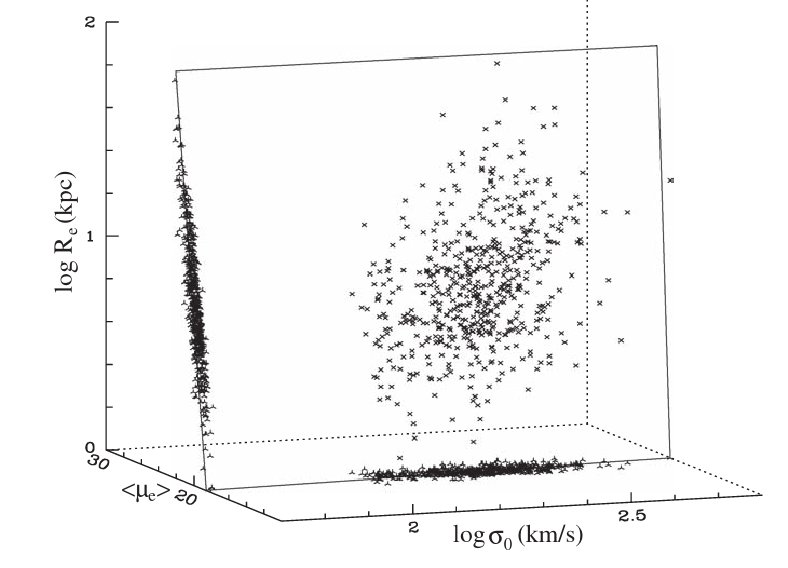
The elliptical galaxies also obey scaling relations between structural parameters and kinematic parameters. The effective radius, the average surface brightness within the effective radius and the velocity dispersion lie on a fundamental plane for elliptical galaxies (see data compiled by MBW book from Saglia et al. 1997, Wegner 1999).
[14]:
Image("images/fundamental_plane.png", width=width)
[14]:
Disk galaxies
As we see in the Hubble tuning fork diagram, disk galaxies are quite complicated with spiral arms, bars, bulges and existence of dust lanes. Ignoring all the complications, at zeroth order, galaxies are axisymmetric. Therefore, one can characterize the disk galaxies with the radially averaged surface brightness distribution and the vertical structure of the disk.
The surface brightness distribution of a number of disk galaxies (see data compilation from MBW) can be fit by
\begin{equation} I(R) = \frac{L}{2\pi R_{\rm d}^2} \exp \left( -\frac{R}{R_{\rm d}}\right) \end{equation}
over a large range of radii.
Compute the effective radius of the galaxy (integrating within \(R_{\rm eff}\) should result in half the light in the total disk) as a function of \(R_{\rm d}\) if it follows the exponential distribution.
[15]:
Image("images/SBdisk.png", width=width)
[15]:
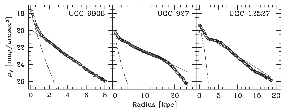
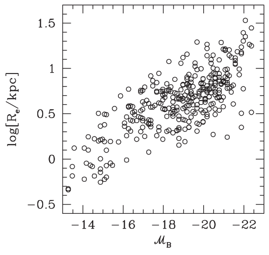
The effective radius scales with the magnitude of the galaxies, with brighter galaxies having larger radii (data compilation in MBW book from Impey et al. 1996b).
[16]:
Image("images/disksSRa.png")
[16]:
Let us look at the deviations in the central region compared to the exponential fit. The central regions show an increase compared to the exponential distribution. These increases can be described by a Sersic profile with a free parameter Sersic index (n) and they correspond to the bulge light light at the center of these galaxies. In the outskirts, some galaxies show another break from the exponential profile. The surface brightness seems to follow an exponential drop with a different scale radius, where the brak radius is a factor few (2.5-4.5) larger than the disk scale length, \(R_{\rm d}\).
Initially it was thought that the bulges would be fit with \(n=4\) (de Vaucouleurs law). Given that the Sersic indices of the bulges can be different, there was and is a discussion about the division of bulges in to classical bulges (n=4) and pseudo bulges (n=1). There is also discussion on whether these differences correspond to the formation mechanisms of bulges. However it is found that bulges have a range of Sersic indices rather than any bimodality.
Here are some examples of scaling relations followed by disk galaxies from the data compilation by Graham 2013.
[17]:
Image("images/disksSR.png", width=width)
[17]:
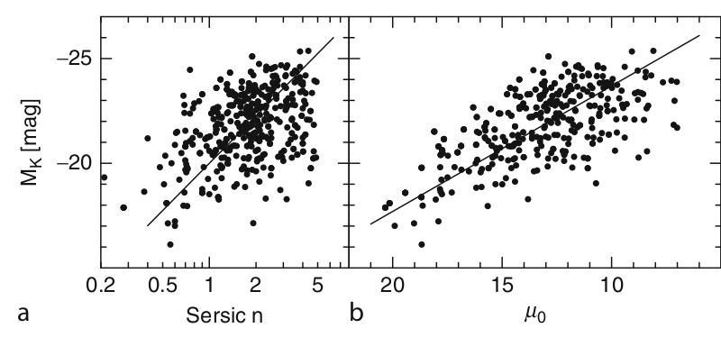
Brighter bulges have large concentrations, and have larger surface brightness. There are also examples of bulgeless galaxies. How these galaxies survive the large amount of merging expected in \(\Lambda\)CDM models, whether the masses of their black holes are correlated with the stellar mass of the entire galaxy are being actively researched.
Galaxy disks which are viewed edge-on also show vertical structure which can be fit by
\begin{equation} f(z) = {\rm sech}^{2/n} \left( \frac{n|z|}{2z_{\rm d}} \right)\,. \end{equation}
Values of \(n=4, 2\) and \(n=\infty\) have been used to fit the vertical structure. These values of \(n\) corresponds to a \({\rm sech}^2\), \({\rm sech}\), and exponentially declining model along the vertical direction.
Plot these distributions as a function of the height z
The distributions often depend upon the behaviour at the mid-plane, larger values of n correspond to steeper profile at the center. The exact behaviour can be difficult to determine from edge on galaxies due to the presence of dust lanes, though.
Bars
The bars seen in spiral galaxies can be characterized using the structure of their isophotes. The projected distribution of these bars can be fit with
\begin{equation} \left(\frac{|x|}{a}\right)^c + \left(\frac{|y|}{b}\right)^c = 1 \end{equation}
with c equal to 2 corresponds to ellipses, while larger values of c give rise to bar like structures.
Plot the above equations for various values of c.
Although vertical heights of bars are quite difficult to determine, based on observations of edge on galaxies with bars, there is evidence that bars are quite thin.
Kinematic scaling relations
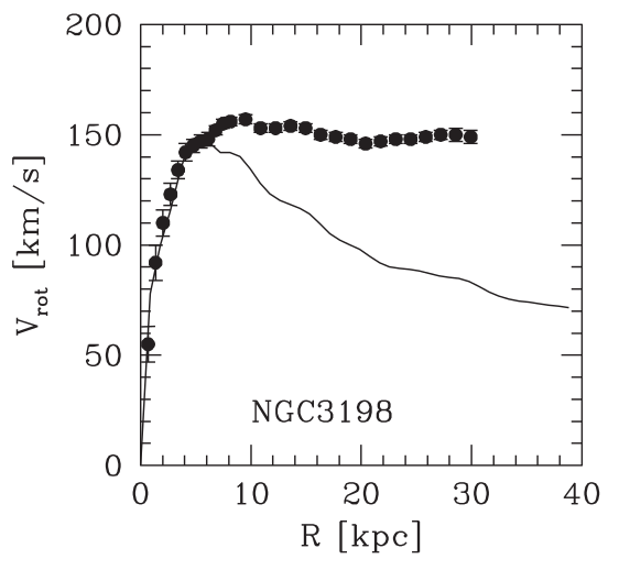
Spectroscopic observations of HII emission regions in disk galaxies (optical disk) or the 21 cm observations of cold gas around galaxies (much further than the optical disk of the galaxy) can be used to measure the velocity field of disk galaxies. The circular orbits in a disk galaxy allow us to use these velocities to infer the rotation curve and thus the mass of the galaxy. For spherically symmetric mass distributions,
\begin{equation} V_{\rm c}^2 (R) = \frac{G M(\lt R)}{R}. \end{equation}
The relation is a bit different for just disks, but far away from the stellar and gas disk one should observe a Keplerian drop off in the rotation velocities. Instead rotation curves show flattening at large radii, showing that the enclosed mass should grow with the radius. This is considered as evidence for dark matter in galaxies.
[18]:
Image("images/Vcirc.png", width=width)
[18]:
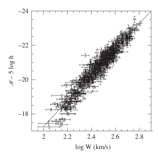
Although the velocity at larger radii is not driven by the luminosity of the galaxy, the maximum circular velocity shows a correlation with luminosity. This is called the Tully Fisher relation. The scatter between the two observables is quite small. In fact it is hard to measure the intrinsic scatter of the relation as the observed scatter seems to be driven by the measurement errors. The figure below (data from Begeman 1989) shows the width of the 21 cm line which is related to twice the maximum circular velocity \(V_{\rm max}\).
[19]:
Image("images/TullyFisher.png", width=width)
[19]: