Orbit theory
Now that we have potential density pairs which satisfy the Poisson equation, we will start to look into orbits in these potentials. We start off with simple point mass located at the origin acting as the source of the potential, and follow the orbit of a test particle in this potential.
Spherical coordinate system
We will use a spherical coordinate system. From simple geoemtrical arguments one can show that
\begin{eqnarray} \hat{r} = \sin\theta\cos\phi \hat{i} + \sin\theta\sin\phi \hat{j} + \cos\theta \hat{k}\\ \hat{\theta} = \cos\theta\cos\phi \hat{i} + \cos\theta\sin\phi \hat{j} - \sin\theta \hat{k}\\ \hat{\phi} = -\sin\theta\sin\phi \hat{i} + \sin\theta\cos\phi \hat{j}\\ \end{eqnarray}
We will often require the derivatives of the unit vectors in spherical coordinate system with respect to time. These can be obtained by differentiating the above with respect to time,
\begin{eqnarray} \frac{d\hat{r}}{dt} = \left[\dot{\theta}\,\hat{\theta} + \sin\theta\,\dot{\phi}\,\hat{\phi}\right]\,,\\ \frac{d\hat{\theta}}{dt} = -\dot{\theta}\, \hat{r}\, + \cos\theta\dot{\phi}\,\hat{\phi} \\ \frac{d\hat{\phi}}{dt} = \sin\theta \dot{\phi} \hat{\theta} - \cos\theta\dot{\phi}\hat{r} \end{eqnarray}
Spherically symmetric potential
The location of the test particle can be specified by its position vector \(r\hat{r}\). The velocity of the particle will be given by differentiating this equation
\begin{equation} \vec{v} = \frac{d (r\hat{r})}{dt} = \dot{r}\,\hat{r} + r\,\left[\dot{\theta}\,\hat{\theta} + \sin\theta\,\dot{\phi}\,\hat{\phi}\right]\,. \end{equation}
The acceleration can be obtained by differentiating the above with respect to time once again.
\begin{equation} \frac{d\vec{v}}{dt} = \left[\ddot{r} - r\dot\theta^2 - r \sin^2\theta\dot\phi^2 \right]\hat{r} + \left[r\ddot{\phi}\sin\theta + 2 \dot{r}\dot{\phi}\sin\theta + 2\dot{r}\dot{\theta}\dot{\phi}\cos\theta\right]\hat{\phi} + \left[r\ddot{\theta} +2\dot{r}\dot{\theta} - r\dot{\phi^2}\sin\theta\cos\theta\right]\hat{\theta} \end{equation}
If we compute the time derivative of \(\vec{r}\times \vec{v}\), we find that
\begin{equation} \frac{d(\vec{r} \times \vec{v})}{dt} = \vec{r} \times \frac{d\vec{v}}{dt} + \vec{v}\times\vec{v} = \vec{r} \times \frac{d\vec{v}}{dt} \end{equation}
For a central force problem (either a point mass or spherically symmetric mass distribution with the center as the origin), we will have the force per unit mass to be in the same direction as the position. Thus the cross product above on the right hand side gives zero. The cross product of \(\vec{r}\) and \(\vec{v}\) defines a direction and since it stays constant during an orbit, it follows that the orbit is planar.
In these cases we can simplify the problem by working on a special coordinate system, where \(\theta=\pi/2\), and then \(r\) and \(\phi\) act as the coordinates on the plane. A rotation of the coordinate system will have to be done for the orbit of each star. Remember that this will not mean the entire system of stars orbiting in this system has to go in the same plane, just that the plane of the orbit of each individual star is going to be planar.
The force per unit mass given by
\begin{eqnarray} \ddot{r} - r \dot\phi^2 &=& -\frac{d\Phi}{dr} \,, \\ r\ddot{\phi} + 2 \dot{r}\dot{\phi} &=& 0 \end{eqnarray}
The second of these equations can be integrated to obtain \(r^2\dot{\phi}=L=\) constant. This when substituted in the first equation removes the \(\phi\) dependence. Thus we obtain
\begin{equation} \ddot{r} - \frac{L^2}{r^3} = -\frac{d\Phi}{dr} \end{equation}
Integrating once with respect to r, gives an equation for \(\dot{r}\). Noting that \(\ddot{r} = \dot{r}d{\dot r}/dr\),
\begin{equation} \frac{1}{2}\dot{r^2} + \frac{L^2}{2r^2} + \Phi(r) = E \end{equation}
which implies
\begin{equation} \frac{dr}{dt} = \pm \sqrt{ 2\left[E-\Phi(r) - \frac{L^2}{2r^2} \right]} \end{equation}
Either signs are possible for the rate of change of \(r\). The points where the velocity equals zero correspond to maximum and minimum radii possible in an orbit.
Qualitatively plot \(L^2/2r^2 + \Phi(r)\) for the point mass potential.
Draw a horizontal line corresponding to an energy \(E\) and show the part of the diagram which an orbit with energy E can occupy.
Suppose this was the potential corresponding to the solar system, where would the planets lie? Where would comets with elliptical orbits lie? Where would comets with hyperbolic orbits lie?
Radial and angular oscillations
One can compute the time required to undergo one oscillation in the radial direction from \(r_{\rm peri}\) to \(r_{\rm apo}\) and back. This can be obtained as twice the integration of the velocity equation from \(r_{\rm peri}\) to \(r_{\rm apo}\) using the positive root.
\begin{equation} T_{\rm radial} = \int_{r_{\rm peri}}^{r_{\rm apo}} \frac{2dr}{\sqrt{2\left[E-\Phi(r)\right] - \frac{L^2}{r^2}}} \end{equation}
During this period, the particle will also move in the azimuthal direction,
\begin{equation} \Delta\phi = \int_0^{T_{\rm radial}} L \frac{dt}{r^2} = 2 \int_{r_{\rm peri}}^{r_{\rm apo}} \frac{Ldr}{r^2}\frac{dt}{dr} = 2 \int_{r_{\rm peri}}^{r_{\rm apo}} \frac{Ldr}{r^2 \sqrt{2\left[E-\Phi(r)\right] - \frac{L^2}{r^2}} } \end{equation}
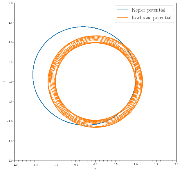
Integrate the above equations for the different potential-density pairs we studied in the previous chapter: point mass, homogeneous sphere and isochrone cases.
Show that for the Kepler potential \(\Delta\phi = 2\pi\) while for the homogeneous sphere \(\Delta\phi=\pi\). This will imply that the orbit will be closed in these cases.
In the case of a generic isochrone potential when \(2\pi/\Delta\phi\) is not rational, the orbit forms a rosette. The orbit will take the particle on an orbit which over time will fill the entire region between the apocenter and the pericenter.
Integrals of motion
A constant of motion is a function of \(f(\vec{r}, \vec{v}, t)\) which is a constant along any orbit in a given potential. For three dimensional motion, any particle will have 6 constants of motion. We know that one can integrate the equations of motion to obtain the \(\vec{r(t)}, \vec{v(t)}\) at any given instant given the initial conditions \(\vec{r(0)}, \vec{v(0)}\). Inverting these equations will give us the initial conditions which are constant. Thus the inverting function would be a constant of motion.
Integrals of motion are special constants of motion which do not depend upon time, but just on the phase space coordinates along the orbit, such that \(I[\vec{x}(t), \vec{v}(t)] =\) constant. Some integrals of motion can be easily expressed in terms of the phase space coordinates, say for example, the energy or angular momentum of an orbit.
The integrals of motion are quite important to reduce the complexity of orbits. For a static spherically symmetric potential, for example, we have the energy (one number) and angular momentum (three numbers) to be integrals of motion. These integrals of motion reduce the dimensionality of the orbits which are possible. In the case of the Kepler potential, there are 5 integrals of motion, and so the dimensionality of the orbit is reduced to just one. The fifth integral of motion corresponds to the angular phase in the plane joining the focus and the pericenter. This reduces the motion in 6-d phase space to collapse to a single dimension. But Kepler potential is a special case: consider for example the spherically symmetric potential
\begin{equation} \Phi(r) = -GM\left[ \frac{1}{r} + \frac{a}{r^2} \right] \end{equation}
For motion in this potential, we start with the radial acceleration equation
\begin{eqnarray} \frac{d^2 r}{dt^2} - \frac{L^2}{r^3} = -GM\left[\frac{1}{r^2} + \frac{2a}{r^3}\right] \end{eqnarray}
Using \(r^2\dot\phi=L\), and substituting \(u=1/r\), we obtain
\begin{eqnarray} -\frac{L^2}{r^2}\frac{d}{d\phi}\left(\frac{1}{r^2}\frac{dr}{d\phi}\right) - \frac{L^2}{r^3} = -GM\left[\frac{1}{r^2} + \frac{2a}{r^3}\right]\\ -L^2u^2 \frac{d^2u}{d\phi^2} - L^2u^3 = -GM\left[ u^2 + 2au^3 \right]\\ -\frac{d^2u}{d\phi^2} - u = -\frac{GM}{L^2}\left[1 + 2au\right]\\ \frac{d^2u}{d\phi^2} + \left(1-\frac{2GMa}{L^2}\right) u = \frac{GM}{L^2}\\ \frac{d^2u}{d(Q\phi)^2} + u = \frac{GM}{Q^2L^2} \end{eqnarray}
The solution of the last equation is
\begin{equation} u = C\cos\left[(\phi-\phi_0)Q \right] + \frac{GM}{L^2Q^2} \end{equation}
with two constants \(C\) and \(\phi_0\). The constant \(C\) is a combination of \(E\) and \(L\)
\begin{equation} C^2 = 2E + \left[\frac{GM}{Q^2L^2}\right]^2\,. \end{equation}
The second constant can be inverted to obtain \(\phi_0\) as a function of \(r, \phi, E\) and \(L\). This gives another integral of motion for this more general case,
\begin{equation} \phi_0 = \phi - \frac{1}{Q}\left(\cos^{-1}\left[\frac{1}{Cr} - \frac{GM}{CL^2Q^2}\right] + 2n\pi \right) \end{equation}
The question arises what this integral signifies exactly and does it simplify our understanding of the orbit? To begin with the orbit is in 6 dimensional phase-space. Suppose we have been given \(L\), \(E\), \(\phi_0\) (corresponding to 5 integrals of motion), and the radial coordinate \(r\), do these numbers give rise to a single (or discrete number of points) \(\phi\) value modulo \(2\pi\)? If Q is a rational number then one can indeed make such a choice by forcing n to be the integral denominator of Q. But for irrational Q, no matter what value of n we choose, we can get arbitrarily close to any value of \(\phi \in [0, 2\pi]\).
This shows that the integral of motion corresponding to \(\phi_0\) is not really that helpful in reducing the dimensions of the available phase space further in the general case. Such integrals of motion are called non-isolating, while those integrals, whose values are once specified, reduce the dimension of the available phase space, are called isolating integrals.
When we decide to compute orbit families for a given potential, we would want to consider doing it as a function of the isolating integrals of motion.
Axisymmetric potentials
For the axisymmetric cases, we should be using the cylindrical coordinate system. The unit vectors in the cylindrical coordinate system are given by
\begin{eqnarray} \hat{R} &=& \cos\theta\,\hat{i} + \sin\theta\,\hat{j}\\ \hat{\theta} &=& \sin\theta\,\hat{i} - \cos\theta\,\hat{j}\\ \hat{z} &=& \hat{k} \end{eqnarray}
The derivatives of these vectors are given by
\begin{eqnarray} \frac{d\hat{R}}{dt} &=& \dot\theta\hat\theta\\ \frac{d\hat{\theta}}{dt} &=& -\dot\theta\hat{R}\\ \frac{d\hat{z}}{dt} &=& 0 \end{eqnarray}
The position vector, velocity vector and acceleration vector will be given by
\begin{eqnarray} \vec{r} &=& R\,\hat{R} + z\,\hat{z} \\ \vec{v} &=& \dot{R}\,\hat{R} + R \dot\theta\,\hat\theta + \dot{z}\,\hat{z}\\ \vec{a} &=& \ddot{R}\,\hat{R} + 2\dot{R} \dot\theta\,\hat\theta + R\ddot{\theta} \hat{\theta} - R\dot\theta^2 \hat{R} + \ddot{z}\,\hat{z}\\ &=& \left(\ddot{R} - R\dot\theta^2\right) \hat{R} + \ddot{z} \hat{z} + \left(2\dot{R} \dot\theta + R\ddot{\theta}\right) \hat{\theta} \end{eqnarray}
Due to axial symmetry, the gradient of the potential is only in the \(R\) and \(z\) direction. Therefore, the component of the acceleration in \(\hat\theta\) direction should equal zero. This implies, \(R^2\dot\theta =\) constant which we define to be \(L_{z}\). The other two components give a coupled equations in the \(R\) and \(z\) plane.
\begin{eqnarray} \ddot{R} &=& -\frac{\partial\Phi}{\partial R} +\frac{L_z^2}{R^3} \\ &=& -\frac{\partial\Phi}{\partial R} -\frac{d}{dR}\left(\frac{L_z^2}{2R^2}\right)\\ \ddot{z} &=& -\frac{\partial\Phi}{\partial z} \end{eqnarray}
Summing the two equations and integrating we obtain
\begin{equation} \frac{1}{2}\left(\dot R^2 + \dot z^2\right) + \Phi_{\rm eff}(R, z) = E \end{equation}
The effective potential includes the gravitational potential plus the energy related to angular momentum. All the orbits of a given energy should lie in a region with \(\Phi_{\rm eff}(R, z)\leq E\).
Let us explore some such orbits in the code below.
[1]:
from galpy import potential
from galpy.orbit import Orbit
from galpy.util import bovy_plot
import numpy as np
[2]:
%pylab inline
figsize(10,10)
# Initialize potential
kepler = potential.KeplerPotential(normalize=1.)
isochrone = potential.IsochronePotential(normalize=1.0, b=1.0)
# Initialize orbit with some starting point
orb = Orbit([1.,0.1,1.1,0.])
orb_iso = Orbit([1.,0.1,1.1,0.])
tstep = numpy.linspace(0.,100.0,10000)
orb.integrate(tstep,kepler) #, method='symplec4_c')
orb_iso.integrate(tstep, isochrone) #, method='symplec4_c')
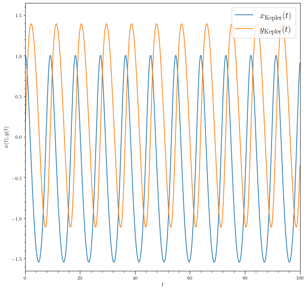
orb.plotx(ylabel=r'$x(t),y(t)$',yrange=[-1.65,1.65],
label=r'$x_{\rm Kepler}(t)$')
orb.ploty(label=r'$y_{\rm Kepler}(t)$',overplot=True)
legend(fontsize=18.,loc='upper right')
orb.plot(label=r'Kepler potential')
orb_iso.plot(label=r"Isochrone potential", overplot=True)
xlim(-2.0, 2.0)
ylim(-2.0, 2.0)
legend(fontsize=18.)
Populating the interactive namespace from numpy and matplotlib
[2]:
<matplotlib.legend.Legend at 0x7fb250b30c40>
findfont: Font family ['serif'] not found. Falling back to DejaVu Sans.
[3]:
#%pylab inline
figsize=(10, 10)
import sys
if not sys.warnoptions:
import warnings
warnings.simplefilter("ignore")
Lz = 1.0
levels= numpy.linspace(-7.25,0.,31)
# Initialize potential
miyamoto = potential.MiyamotoNagaiPotential(normalize=True, b=0.1)
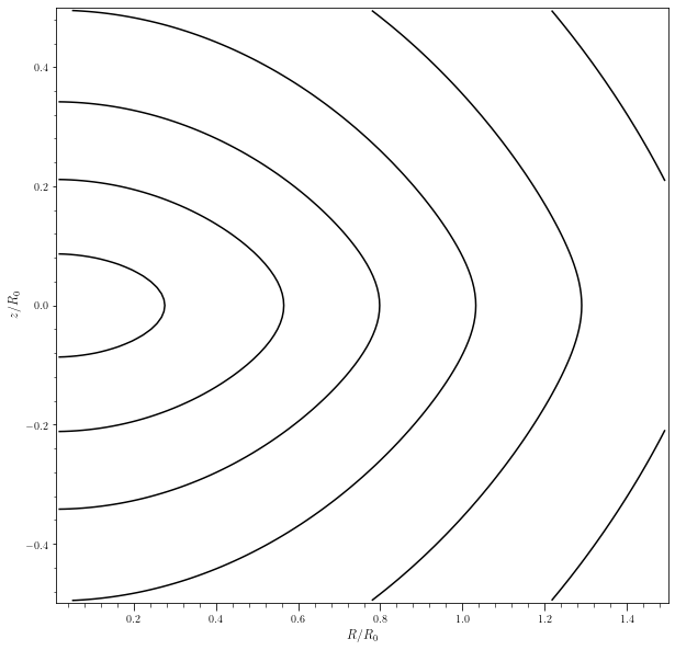
tmp = potential.plotPotentials(miyamoto, rmin=.01,nrs=101,nzs=101,
justcontours=True,
levels=levels,
effective=False,
Lz=Lz)
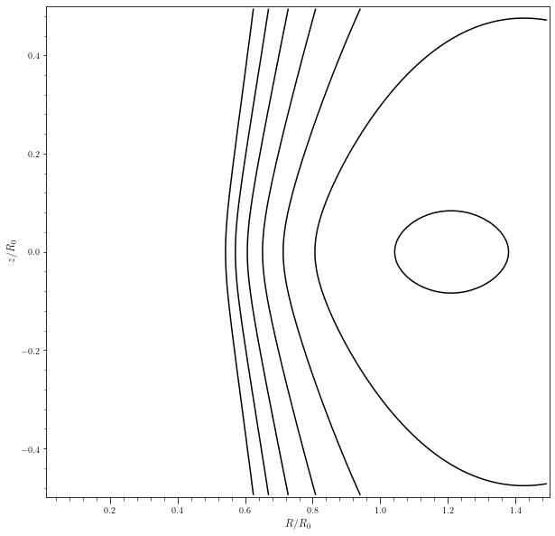
[4]:
tmp = potential.plotPotentials(miyamoto, rmin=.01,nrs=101,nzs=101,
                         justcontours=True,
                         levels=levels,
                         effective=True,
                         Lz=Lz)
scatter([1.0], [0], color="red", label="Guiding radius")
legend(fontsize=18.0)
[4]:
<matplotlib.legend.Legend at 0x7fb2793d8070>
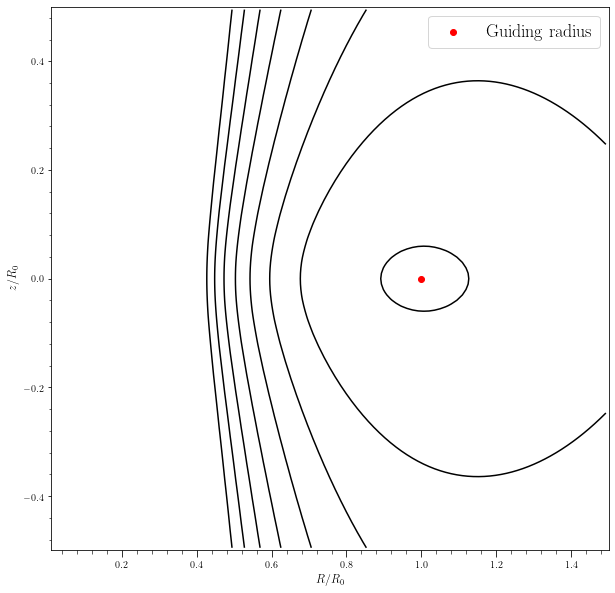
Now let us see the effective potential for an orbit with a larger value of \(L_z\). We keep the same contour levels, so the contours will be expected to shift towards the right, and the guiding radius corresponding to the circular orbit will move further out.
[5]:
Lz = 1.25
tmp = potential.plotPotentials(miyamoto, rmin=.01,nrs=101,nzs=101,
                         justcontours=True,
                         levels=levels,
                         effective=True,
                         Lz=Lz)
[6]:
# Now let us integrate orbits.

def orbit_RvRELz(R,vR,E,Lz,pot=None):
    """Returns Orbit at (R,vR,phi=0,z=0) with given (E,Lz)"""
    return Orbit([R,vR,Lz/R,0.,
                  numpy.sqrt(2.*(E-potential.evaluatePotentials(pot,R,0.)
                                 -(Lz/R)**2./2.-vR**2./2)),0.])

R, E, Lz= 0.8, -1.45, 1.0
vR= 0.
o1= orbit_RvRELz(R,vR,E,Lz,pot=miyamoto)
ts= numpy.linspace(0.,1000.,100001)
o1.integrate(ts, miyamoto)
o1.animate()
[6]:
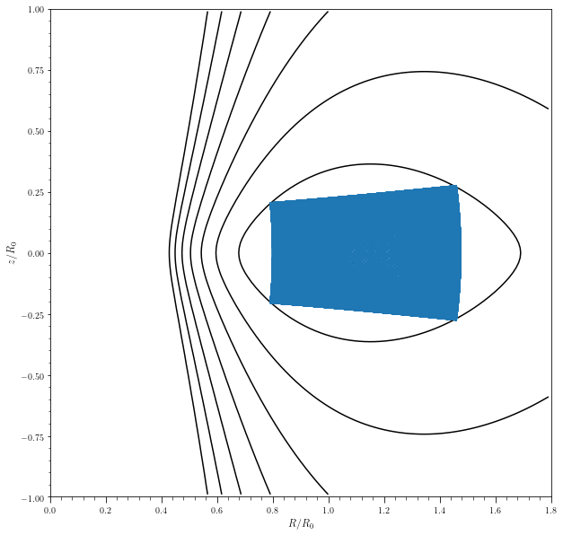
[7]:
tmp = potential.plotPotentials(miyamoto,
                         rmin=0.0,rmax=1.8,
                         zmin=-1.0,zmax=1.0,
                         nrs=101,nzs=101,
                         justcontours=True,
                         levels=levels,
                         effective=True,
                         Lz=Lz)

o1.plot(overplot=True)
[7]:
[<matplotlib.lines.Line2D at 0x7fb2786ccd90>]
[8]:
R, E, Lz= 0.8, -1.45, 1.0
vR= 0.5
o2= orbit_RvRELz(R,vR,E,Lz,pot=miyamoto)
o2.integrate(ts, miyamoto)
[9]:
R, E, Lz= 1.0, -1.45, 1.0
vR= 0.0
o3= orbit_RvRELz(R,vR,E,Lz,pot=miyamoto)
o3.integrate(ts, miyamoto)
[10]:
R, E, Lz= 0.98, -1.7, 1.0
#R, E, Lz= 1.1, -1.45, 1.0
vR= 0.0
o4= orbit_RvRELz(R,vR,E,Lz,pot=miyamoto)
t4 = numpy.linspace(0.,400.,4001)
#t4= numpy.linspace(0.,15.,1001)
o4.integrate(t4, miyamoto)
o4.animate()
[10]:
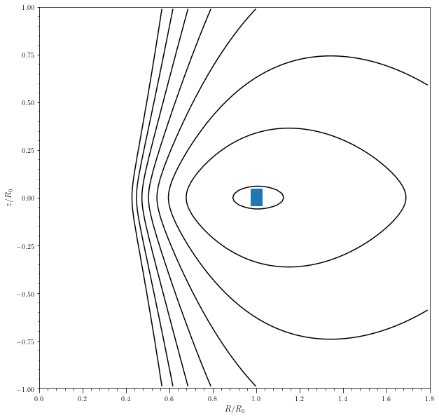
[11]:
tmp = potential.plotPotentials(miyamoto,
                         rmin=0.0,rmax=1.8,
                         zmin=-1.0,zmax=1.0,
                         nrs=101,nzs=101,
                         justcontours=True,
                         levels=levels,
                         effective=True,
                         Lz=Lz)

#o1.plot(overplot=True)
#2.plot(overplot=True)
#o.plot(overplot=True)
o4.plot(overplot=True)
[11]:
[<matplotlib.lines.Line2D at 0x7fb278b78700>]
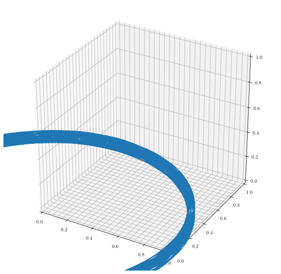
[12]:
ax = subplot(111, projection="3d")
#o1.plot3d(overplot=True)
#o2.plot3d(overplot=True)
#o3.plot3d(overplot=True)
o4.plot3d(overplot=True)
ax.view_init(30)
There is an entire phase space area which is available inside the second black contour which is energetically available to the particle, and yet these two orbits seem to occupy a different part of the phase space. In disk potentials, we get a third integral of motion in addition to \(E\) and angular momentum, \(L_z\). The orbits displayed above have a different value for this third integral of motion.
Writing down this integral is quite tedious, but there is another tool which can be used to identify these integrals of motion, introduced by Henri Poincare - surfaces of section.
Develop intuition by playing with the orbits above in these different potentials.
Use prolate and oblate potentials and then look at the orbits by using the above piece of code.
Surfaces of section
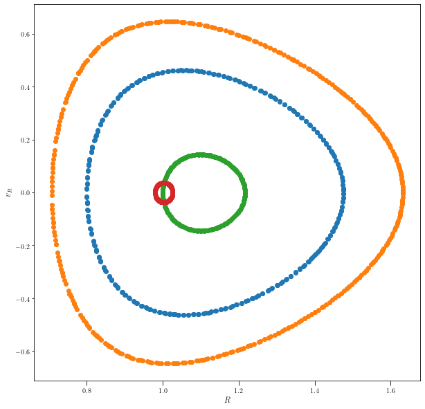
Surfaces of section can be used to show that indeed a third integral of motion exists for many of these orbits. In the meridional plane, we start with a total of 4 phase space coordinates. The energy of a given particle, can be used to get rid of one phase space coordinate, say \(\dot z\), reducing the dimension of available phase space to 3. Now let us consider the intersection of this three dimensional surface with the plane \(z=0\). This will be some two dimensional surface in the \((R, v_R)\) plane.
For every orbit, one can make a scatter plot of points in this plane, when the value of z is close to zero. We observe that many of these orbits do not cover a two dimensional surface in the \((R, v_R)\) plane but instead a curve even after many orbits. This shows that there is a non-classical third integral of motion for these orbits.
Code for surfaces of section
[13]:
def sos(R,z,vR):
    sign1 =np.sign(z[1:])
    sign2 = np.sign(z[:-1])
    idx = (sign1*sign2 == -1) & (sign2<0)
    return (R[1:][idx],vR[1:][idx])

sos_R,sos_vR=sos(o1.R(ts),o1.z(ts),o1.vR(ts))
scatter(sos_R,sos_vR)

sos_R,sos_vR=sos(o2.R(ts),o2.z(ts),o2.vR(ts))
scatter(sos_R,sos_vR)

sos_R,sos_vR=sos(o3.R(ts),o3.z(ts),o3.vR(ts))
scatter(sos_R,sos_vR)

# This orbit has a different Energy E
sos_R,sos_vR=sos(o4.R(t4),o4.z(t4),o4.vR(t4))
scatter(sos_R,sos_vR)

#scatter([1.1], [0], color="red", label="Guiding radius")


xlabel(r'$R$')
ylabel(r'$v_R$')
[13]:
Text(0, 0.5, '$v_R$')
Orbits near the guiding radius
The orbits that we discussed above are very useful to understand the dynamics in prolate and oblate potentials. However, most of the stars in disk galaxies are moving at velocities which are close to the circular velocities within the disk. The orbits thus have energies very close to what is required to be at the guiding radius. Therefore it is useful to study such orbits as well.
We can define a new variable \(x=R-R_{\rm g}\). The effective potential close to the guiding radius and close to the midplane \(z=0\) can be written down by performing a Taylor expansion,
\begin{equation} \Phi_{\rm eff}(x, z) = \Phi_{\rm eff}(R_{\rm g}, 0) + \left.\frac{1}{2}\frac{\partial^2 \Phi_{\rm eff}}{\partial R^2}\right|_{(R_{\rm g}, 0)} x^2 + \left.\frac{1}{2}\frac{\partial^2 \Phi_{\rm eff}}{\partial z^2}\right|_{(R_{\rm g}, 0)} z^2 + {\cal O}(xz^2) \,. \end{equation}
These equations thus lead to a set of decoupled equations
\begin{eqnarray} \ddot{x} &=& -\kappa^2 x \\ \ddot{z} &=& -\nu^2 z \end{eqnarray}
where the constant \(\kappa\) and \(\nu\) are defined to be
\begin{eqnarray} \kappa^2 &=& \left.\frac{\partial^2\Phi}{\partial R^2}\right|_{R_{\rm g}, 0} + \frac{3L_z^2}{R_{\rm g}^4}\\ \nu^2 &=& \left.\frac{\partial^2\Phi}{\partial z^2}\right|_{R_{\rm g}, 0} \end{eqnarray}
The frequencies \(\kappa\) and \(\nu\) are called the epicycle and the vertical frequency, respectively. These frequencies are related to the circular frequency \(\Omega\) in the mid-plane, such that
\begin{equation} R \Omega^2(R) = \left.\frac{\partial \Phi}{\partial R}\right|_{R, 0} = \frac{L_{z}^2}{R^3}\\ \kappa^2 = \left(R\frac{d\Omega^2}{dR} + 4 \Omega^2 \right)_{R_{\rm g}} \end{equation}
For the very inner regions, where the circular velocity grows linearly as a function of radius (i.e. constant \(\Omega\)), we have \(\kappa = 2\Omega\). In general the value of \(\kappa\) lies between \([1, 2]\Omega\).
These equations show that the orbits just close to the guiding radius will have oscillations in the radial direction around the guiding radius, and independent oscillations along the z-direction.
\begin{eqnarray} x = R(t) - R_{\rm g} &=& X \cos\left(\kappa t + \psi \right)\\ z &=& Z \cos\left( \nu t + \zeta \right) \end{eqnarray}
The angular coordinate \(\phi\) can be obtained by integrating the equation for \(\dot{\phi}=L_z/R^2\).
\begin{eqnarray} \int d\phi = \int dt \frac{L_z}{R^2} &=& \int dt \frac{L_z}{(x+R_{\rm g})^2}\\ &\simeq& \int dt \frac{L_z}{R_{\rm g}^2}\left( 1 - 2\frac{x}{R_{\rm g}} \right)\\ \phi(t) &=& \phi_0 + \Omega t - 2\frac{X\Omega}{\kappa R_{\rm g}}\sin\left(\kappa t + \psi \right) \end{eqnarray}
This implies that the orbit of a particle near the guiding radius can be represented with motion on an ellipse centered on the circular orbit at the guiding radius. This will still create rosette orbits in the mid-plane.