Gravitation
The gravitational force is the dominant force that shapes the structure of galaxies. So we will go through some of the basics of gravitation, and see how the concepts we learn can be applied to galaxies. Einstein’s general theory of relativity represents our current best understanding of gravity. Einstein’s equations:
\begin{equation*} G_{\mu\nu} = 8 \pi G T_{\mu\nu}\,. \end{equation*}
The tensor \(G_{\mu\nu}\) contains the second derivatives of the metric components, and in the weak field, small velocity limit, the deviations of the metric from the Minkowski metric come in the form of \(\Phi/c^2\). The field equations of GR were derived such that they reduce to Newtonian gravity in such a limit, and reduce to the familiar Poisson equation
\begin{equation*} \nabla^2 \Phi = 4 \pi G \rho \end{equation*}
The mass distribution within an object can be specified by the density, \(\rho\). The solution to the above equation will then determine the potential \(\Phi\). The potential then specifies the forces that will act on test particles, and thus determine their orbits.
\begin{equation*} \vec{F} = -m \nabla \Phi \end{equation*}
The orbits of test bodies in the galactic potential are observable. Thus our goal would be to compare observations to the orbits predicted from the solutions of the Poisson equation above. Agreement would imply that the Poisson equation which is so well tested in the solar system works also on galactic scales. Disagreement could be a result of anamolous terms on either side of the Poisson equation. A change to the left hand side would imply a change in our understanding of gravity, while a change to the right hand side would imply a missing link in our understanding of matter which contributes the gravitational force.
Time scales important for dynamics
Let us look at order of magnitudes of some important time scales for galactic dynamics.
Hubble time scale:
The Hubble parameter is of the order \(H_0\)~100 km/s/Mpc. This gives a time scale for the Universe of order 1/H0, which is close to \(10^{10}\) years.
Orbital time scale:
The orbital time scale can be obtained simply as,
\begin{equation} t_{\rm orb} \sim 2\pi R/v_{\rm circ} \end{equation}
The circular velocity for Milky Way flattens and reaches a value close to 200 \({\rm kms}^{-1}\). The orbital time scale for the rotation at the position of the Sun (10 kpc) is about \(10^8\) years. Thus the Milky way would make many rotations within the age of the Universe, and we can assume that it should be in dynamical equilibrium. If you compute the orbital time scales close to the edge of the dark matter halos, these come out to be comparable to the Hubble time scale, so the assumption of dynamical equilibrium may not be appropriate on those scales.
Direct collision time scale:
The mean free path of particles within the galaxy can be computed as \(\lambda \sim 1/(n\sigma)\), where \(n\) is the number density of stars and \(\sigma\) the cross section for direct collisions of stars. The collision time scales will then be given by
\begin{equation} t_{\rm direct} \sim \lambda/v \sim R^3/R_{\odot}^2/N/v \sim t_{\rm orb} (R/R_{\odot})^2/N \end{equation}
For the Milky Way, the average number density of stars in the galaxy is about 1 star per parsec cubed (\(10^{11}\) stars within a disk of 10 kpc with 1 kpc thickness), and the cross section is \(4 \pi R_\odot^2\), assuming all stars in the galaxy to be like the Sun. This mean free path then turns out to be \(\lambda \sim 1.5\times10^{11}\) kpc, which is orders of magnitude larger than the path length within a single orbit. With velocities of the order \(100 kms^{-1}\), the collision time scale is quite large even compared to the Hubble time scale and stellar collisions within the galaxy should be exceedingly rare.
Relaxation time scale:
Direct collisions are rare, but particles can change their velocities due to long range interactions. The time scale over which a particle changes its velocity by factor of order unity is called the relaxation time scale. The effect of an encounter of a particle with another particle of mass m with an impact parameter b and moving with velocity v is to change its velocity by
\begin{equation} \Delta v_\perp \sim 2Gm/(bv) \end{equation}
The particle will encounter all sort of impact parameters during its motion through the galaxy. The number of impacts between \(b\pm db\) will be \(2 \pi b db N/(\pi R^2)\). Thus the cumulative kicks it will gather within an orbital time will be
\begin{eqnarray} |\Delta v_\perp^2| &=& \int_{R_{\rm min}}^{R} \left(\frac{2Gm}{bv}\right)^2 \frac{2 \pi b db N}{\pi R^2} \, &=& \left(\frac{2Gm}{v}\right)^2 2 \ln \left(\frac{R}{R_{\rm min}}\right) \frac{N}{R^2} \, \end{eqnarray}
The value of \(R_{\rm min}\)
\begin{equation} R_{\rm min} \sim \frac{2Gm}{v^2} \sim \frac{2GM}{v^2N} \sim \frac{R}{N} \end{equation}
would determine the scale where the velocity kicks become comparable directly to the typical velocity. Thus, within one orbital time through the galaxy, the velocity kicks will accumulate energy proportional to
\begin{equation} |\Delta v_\perp^2| = \left(\frac{2GM}{v}\right)^2 2 \frac{\ln N}{N} \frac{1}{R^2} = \left(\frac{GM}{v}\right)^2 8 \frac{\ln N}{N} \frac{1}{R^2} \end{equation}
Equating these to the energy of the particle per mass, we get a value for the relaxation time
\begin{equation} t_{\rm relax} \sim \frac{R}{v} \frac{v^2}{|\Delta v_\perp^2|} \sim \frac{R}{v} \frac{v^2}{\left(\frac{GM}{v}\right)^2 8 \frac{\ln N}{N} \frac{1}{R^2} } \sim t_{\rm orb} \left[\frac{N}{8\ln N}\right] \end{equation}
For a system with size of the Milky way, \(N \sim 10^{11}\), which corresponds to about \(10^{17}\) years!
Close encounter time scale
The close encounter time scale can be obtained by putting \(R_{\rm min}\) instead of \(R_{\odot}\) in the direct collision time scale.
\begin{equation} t_{\rm close} \sim t_{\rm orb} (R/R_{\rm min})^2/N \sim N t_{\rm orb}\,. \end{equation}
For a system of size of the Milky way, this time scale is close to \(10^{19}\) years, even larger than the relaxation time scale.
[1]:
import numpy as np

class timescales:
    def __init__(self, N, mass, radius, Rmin, H0):
        self.gee = 4.2994e-9

        # Unitless
        self.N = N

        # In Msun
        self.mass = mass

        # In Mpc
        self.radius = radius

        # In km/s/Mpc
        self.H0 = H0

        # Mpc s/km in Gyr
        self.Mpc_s_by_km_to_year = 9.778e2

        # Rmin
        self.Rmin = Rmin

        # velocity
        self.v = np.sqrt(self.gee*self.mass/self.radius)
        print("Velocity:", self.v, "km/s")

        print("Orbital timescale:", self.torb(), "Gyr")
        print("Hubble timescale:", self.tHubble(), "Gyr")
        print("Relaxation timescale:", self.trelax(), "Gyr")
        print("Close interaction timescale:", self.tclose(), "Gyr")
        print("Direct collision timescale:", self.tdirect(), "Gyr")
        print ("==========================")

    def tHubble(self):
        # Return in Gyr
        return 1/self.H0 * self.Mpc_s_by_km_to_year

    def torb(self):
        # Return in Gyr
        return 2*self.radius/self.v * self.Mpc_s_by_km_to_year

    def tdirect(self):
        # Return in Gyr, assumes the radius to be Rsun
        return self.torb()*(self.radius/self.Rmin)**2/self.N

    def tclose(self):
        # Return in Gyr
        return self.torb()*self.N

    def trelax(self):
        # Return in Gyr
        return self.torb()*self.N/8/np.log(self.N)

Rsun_to_Mpc = 1./4.435e13
mwbaryons = timescales(1e11, 1e11, 0.01, Rsun_to_Mpc, 70.0)
globular = timescales(1e4, 1e4, 1e-5, Rsun_to_Mpc, 70.0)
cluster = timescales(1e3, 1e14, 1, 0.010, 70.0)

# Mass of dark matter particle assuming primordial black holes
mdm = 1e-10

# Interaction cross section of about 1 cm^2/gm
rdm = (1*mdm)**0.5*3.24e-25

mwdmhalo = timescales(1e22, 1e12, 0.3, rdm, 70.0)
Velocity: 207.3499457439042 km/s
Orbital timescale: 0.09431398657877353 Gyr
Hubble timescale: 13.968571428571428 Gyr
Relaxation timescale: 46545504.47438488 Gyr
Close interaction timescale: 9431398657.877354 Gyr
Direct collision timescale: 185508302266.48767 Gyr
==========================
Velocity: 2.0734994574390413 km/s
Orbital timescale: 0.009431398657877356 Gyr
Hubble timescale: 13.968571428571428 Gyr
Relaxation timescale: 1.2800013730455844 Gyr
Close interaction timescale: 94.31398657877355 Gyr
Direct collision timescale: 185508302266.4878 Gyr
==========================
Velocity: 655.6981012630737 km/s
Orbital timescale: 2.9824701279947594 Gyr
Hubble timescale: 13.968571428571428 Gyr
Relaxation timescale: 53.96959662622539 Gyr
Close interaction timescale: 2982.4701279947594 Gyr
Direct collision timescale: 29.824701279947593 Gyr
==========================
Velocity: 119.71354699169737 km/s
Orbital timescale: 4.900698498564149 Gyr
Hubble timescale: 13.968571428571428 Gyr
Relaxation timescale: 1.209287679203387e+20 Gyr
Close interaction timescale: 4.900698498564149e+22 Gyr
Direct collision timescale: 4.2015590694137074e+36 Gyr
==========================
Given the long range nature of gravity, one has to compute the potentials by summing over all the other stars. Since the number of stars in a galaxy are quite big, one can consider smooth potentials instead of discrete summation over all the stars.
Our goal in galactic dynamics is to use kinematic observables to understand the density distribution in galaxies. The observables we have is the light coming from galaxies projected on the plane of the sky, and the line of sight velocity at pixelated locations of the galaxy. From these we need to construct the density distribution of the galaxy. The only way forward is to forward model the system. Make an ansatz about the density distribution in the galaxy, obtain the projected light distribution assuming a mass to light ratio. Obtain the potential corresponding to the density distribution. Construct orbits in this potential. Give appropriate weights to orbits and see if they can reconstruct the density distribution.
This goal is quite hefty, so let us start with something very simple to begin with. Galaxies show a variety of symmetries, we will solve the Poisson equation for simpler symmetric density fields. We will start of with simple spherically symmetric mass distributions, and slowly work our way towards more complicated distributions.
Density potential pairs:
Point mass distribution
Let us consider the simple case of the point mass distribution. Let us choose our coordinate system such that the mass is located at the origin (\(\rho(\vec{r}) = M\delta(\vec{r})\)). We seek solutions of the Poisson equation for this density distribution.
One can show that the function \(\nabla^2 |\vec{r}|^{-1}\) is zero for all \(|\vec{r}|\ne 0\). To compute its value at \(\vec{r}=0\), one can consider a small sphere centered at the origin with radius \(R\). The integral
\begin{equation*} \int_{V} \nabla.\nabla \frac{1}{|\vec{r}|} dV = \int_{S} \nabla \frac{1}{|\vec{r}|} . d\vec{A} = -4 \pi \end{equation*}
This implies we can write \(\nabla^2 |\vec{r}|^{-1}= -4\pi \delta(\vec{r})\), and therefore
\begin{equation*} \Phi = -\frac{GM}{|\vec{r}|} \end{equation*}
is indeed a solution of the Poisson’s equation for a delta function density. These two functions \(\left[M\delta(\vec{r}), -GM|\vec{r}|^{-1}\right]\) form a potential and density pair which satisfies the Poisson equation.
The force is just the gradient of the potential, and thus is given by
\begin{equation*} F(\vec{r}) = -\nabla \Phi = -\frac{GM}{|\vec{r}|^3}\vec{r} \end{equation*}
It is also easy to see that if there are two potential density pairs then any linear combination of the two will also form potential density pair. This makes some of the analytical potential density pairs quite useful to study.
For a generic mass distribution \(\rho(\vec{r})\) we should be able to show that
\begin{equation*} \Phi(\vec{r}) = -\int \frac{G\, \rho(\vec{r'})\, d^3\vec{r'}}{\left|\vec{r}-\vec{r'}\right|} \end{equation*}
A lot of things get simplified for spherically symmetric mass distribution which help us to quickly compute the potentials. The Newton’s theorems make it easier to compute these quantities.
Newton’s theorems
Newton’s first theorem
A spherical shell of matter does not exert any gravitational force on bodies that lie anywhere inside (the gravitational potential inside the shell of a given radius is constant).
Newton’s second theorem
The gravitational force on a body lying outside a spherical shell of matter with mass \(M\) is the same as the force exerted due to mass \(M\) lying at the center of the shell.
These theorems are easiest to prove using the Poisson equation integrated over suitable volumes. They also provide a useful way to compute the potentials when combined with the result for the point mass potential above. For a spherical shell of matter with radius \(R\) centered at the origin, we can therefore write down,
\begin{equation} \Phi(\vec{r}) = -\frac{GM}{|\vec{r}|} \,\,\,\,\, \forall \,\, r \geq R \end{equation}
\begin{equation} \Phi(\vec{r}) = -\frac{GM}{R} \,\,\,\,\, \forall \,\, r \leq R \end{equation}
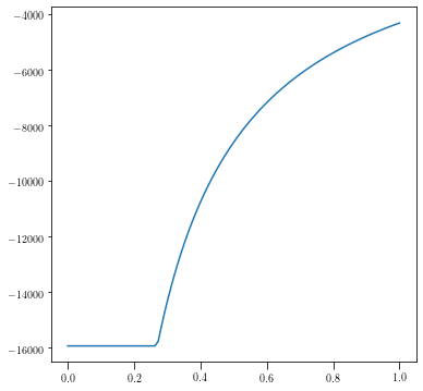
We can plot the gravitational potential due to such a shell.
[2]:
import pylab as pl
%pylab inline
conf = %config InlineBackend.rc
conf['figure.figsize'] = (6, 6)
conf['savefig.dpi']=100
conf['font.serif'] = "Computer Modern"
conf['font.sans-serif'] = "Computer Modern"
conf['text.usetex']=True

%config InlineBackend.rc
%pylab inline
Populating the interactive namespace from numpy and matplotlib
Populating the interactive namespace from numpy and matplotlib
[3]:
class shell:
    def __init__(self, M, R):
        self.Rshell = R
        self.Mass = M
        # Put gravitational constant * mass of the sun /(km/s)^2 /Mpc in google search!
        # What are the units of this constant?
        self.gee = 4.3022e-9

    def potential(self, r):
        if np.isscalar(r):
            r = np.array([r])
        pot = r * 0.0
        idx = r<self.Rshell

        pot[idx] = -1/self.Rshell

        pot[~idx] = -1/r[~idx]

        return pot*self.gee*self.Mass

# Mass in hinv Msun, shell radius in hinv Mpc
Mass = 1e12
sh = shell(1e12, 0.270)
R = np.linspace(0.0, 1.0, 100)

plot(R, sh.potential(R))

# Label the axis of these plots
[3]:
[<matplotlib.lines.Line2D at 0x7f6c0f9c2490>]
A spherically symmetric mass distribution can be decomposed in to smaller shells, and the potential can then be added up. Thus for a density distribution which depends only on the radius, \(\rho(r)\), we obtain
\begin{equation} \Phi(\vec{r}) = -4\pi G \left[\int_r^{\infty} \rho(r') r' dr' + \frac{1}{r}\int_0^{r} \rho(r') r'^2 dr'\right] \end{equation}
This can be shown to be equal to
\begin{equation} \Phi(\vec{r}) = -G \left[\int_{r}^{\infty} \frac{1}{r'^2} M(\lt r') dr'\right] \end{equation}
Circular velocity
Given the potential, one can calculate the velocity of circular orbits
\begin{equation} v_{\rm c}(r) = \sqrt{\frac{GM(\lt r)}{r}} \end{equation}
One can also compute a dynamical time estimate, this is the time required to cross the system. It can be calculated as \begin{equation} t_{\rm dyn} = \frac{2\pi r}{v_c} \propto \frac{1}{\sqrt{G\rho}} \end{equation} There are a number of ways to define dynamical time but all of these will come out to be proportional to \(1/\sqrt{G\rho}\).
Compute the circular velocity of gas particles in a Milky way halo. Assume mass of the Milky way is \(10^{12} h^{-1}M_{\odot}\) halo and compute the velocity at \(0.1\) Mpc from the center which is about 10 times further than the galactocentric distance of the Sun.
Compute the dynamical time at the same distance
Spherically symmetric distributions
Uniform sphere
For a uniform homogeneous sphere with constant density, \(\rho_0\) and radius \(R\),
\begin{eqnarray} \rho(r) = \rho_0 \,\,\,\,\forall\,\,r\lt R \ \rho(r) = 0 \,\,\,\,\forall\,\,r\gt R\,. \, \end{eqnarray}
The potential is given by
\begin{equation} \Phi(r) = - \frac{4\pi G\rho}{3}\frac{ R^3}{r} \,\,\,\,\forall\,\,r\gt R \ \end{equation} \begin{equation} \Phi(r) = - \frac{4\pi G\rho}{3}\frac{ 3R^2-r^2}{2} \,\,\,\,\forall\,\,r \leq R\,. \, \end{equation}
The circular velocity will increase linearly with the radius for \(r \leq R\), \begin{equation} v_c(r) = \sqrt{\frac{4\pi G \rho}{3}} r \,\,\,\,\forall\,\, r\leq R\,. \end{equation} and it falls off as \(r^{-1/2}\) for \(r\gt R\). If there is a disk of test particles moving in a uniform density sphere, then this disk will rotate with a constant angular speed \(\omega=v_{\rm c}/r=\)constant like a solid body.
The dynamical time on the other hand for the system will be constant in these inner regions where the density is uniform, \begin{equation} t_{\rm dyn}(r) = \sqrt{\frac{3\pi}{G \rho}} \,\,\,\,\forall\,\, r\leq R\,. \end{equation} Thus the orbital time period of particles are also independent of the radius in regions of uniform density.
Next let us consider a couple of potentials which smoothly interpolate between the point mass Kepler potential and the homogeneous sphere - Plummer sphere and the isochrone.
Plummer sphere
Let us consider the Plummer sphere where the potential is smoothed in the inner regions compared to the point mass potential.
\begin{equation} \Phi(r) = - \frac{GM}{\sqrt{r^2+b^2}} \ \end{equation}
The Plummer model is often used to compute the potentials of particles in numerical simulations. The smoothing at small scales avoids large forces during close chance interactions. These happen in numerical simulations due to finite mass resolution, but such collisions are expected to play a very insignificant role for large astrophysical systems like galaxies (globular clusters are different).
The density corresponding to this potential can be found by using the Poisson equation and it corresponds to
\begin{equation} \rho(r) = \frac{3M b^2}{4 \pi}\frac{1}{[r^2+b^2]^{5/2}} \end{equation}
The circular velocity will be given by \begin{equation} v_{c}(r) = \sqrt{\frac{GM}{(b^2+r^2)^{3/2}}} \end{equation}
Isochrone potential
Yet another useful potential is the isochrone potential where,
\begin{equation} \Phi(r) = - \frac{GM}{b+\sqrt{r^2+b^2}} \ \end{equation}
By taking the limits \(b\rightarrow 0\), or \(r\rightarrow 0\), one can smoothly interpolate between a point mass potential and the potential of a homogeneous sphere.
Compute the behaviour of the density distribution corresponding to the isochrone at small radii \(r\lt b\).
Compute the behaviour of the density distribution corresponding to the isochrone potential at large radii \(r\gt b\).
The density associated with the potential can be shown to be
\begin{equation} \rho(r) = M \frac{3(b+a)a^2-r^2(b+3a)}{4\pi (b+a)^3a^3} \end{equation}
where \(a=\sqrt{b^2+r^2}\).
Power law density profiles
Many galaxies have density profiles which fall off as \(r^{-\alpha}\). The spherically symmetric version for such a system would be,
\begin{equation} \rho(r) = \rho_0 \left(\frac{r_0}{r}\right)^\alpha \end{equation}
The mass within the radius \(r\) is given by
\begin{equation} M(\lt r) = \int_0^r \rho(r') 4 \pi r'^2 dr' = \frac{4\pi \rho_0 r_0^{3}}{(3-\alpha)} \left(\frac{r_0}{r}\right)^{\alpha-3}\,. \end{equation}
The mass outside the radius \(r\) is given by
\begin{equation} M(\gt r) = \int_r^\infty \rho(r') 4 \pi r'^2 dr' = \frac{4\pi \rho_0 r_0^{3}}{(\alpha-3)} \left(\frac{r_0}{r}\right)^{\alpha-3}\,. \end{equation}
You will see that depending upon the magnitude of \(\alpha\) compared to 3, you either have a infinite enclosed mass or a infinite mass beyond radius \(r\). Clearly such cases are not possible. One needs to have \(\alpha \lt 3\) in the inner regions and \(\alpha \gt 3\) in the outskirts.
Assuming \(\alpha\lt 3\) to avoid divergence of mass at the center, the circular velocity curve is
\begin{equation} v_{\rm circ}^2(r) = \frac{G 4\pi \rho_0 r_0^{3}}{(3-\alpha)} \left(\frac{r_0}{r}\right)^{\alpha-3}\frac{1}{r} \end{equation}
For \(\alpha=2\), we get a flat rotation curve. For \(\alpha=0\), we get the homogeneous sphere, which gives an increase in the circular velocity with radius.
The potential of the system can be computed to be equal to
\begin{equation} \Phi(r) = \begin{cases} \frac{4\pi G\rho_0 r_0^\alpha}{(\alpha-2)(\alpha-3)} r^{2-\alpha}, \,\,\,&& {\rm if}\ 2\lt\alpha\lt 3 \\ \infty \,\,\,&&{\rm otherwise}\,. \end{cases} \end{equation}
Double power law models
Given that single power law density profiles cannot be realistic, we will now consider double power law models. There is a whole family of such models
\begin{equation} \rho(r) = \frac{\rho_0}{\left(\frac{r}{r_{\rm s}}\right)^{\gamma}\left(1 +\left[\frac{r}{r_{\rm s}}\right]^{\alpha}\right)^{(\beta-\gamma)/\alpha}} \end{equation}
We have already encountered one such model previously, \(\alpha=2, \beta=5, \gamma=0\), the Plummer sphere. But there are many others which obey the conditions that the logarithmic slope \(\alpha \lt 3\) in the inner regions and \(\alpha \gt 3\) in the outskirts.
\(\alpha\) |
\(\beta\) |
\(\gamma\) |
Profile |
|---|---|---|---|
2 |
5 |
0 |
Plummer sphere |
1 |
3 |
1 |
NFW profile |
1 |
4 |
2 |
Jaffe profile |
1 |
4 |
1.5 |
Moore profile |
2 |
2 |
0 |
Cored isothermal profile |
2 |
3 |
0 |
Modified Hubble profile |
The logarithmic slope of the density profile at small radii is \(-\gamma\) while that at large radii is \(-\beta\). The third parameter defines how sharp the transition between these two ranges is.
The Navarro Frenk and White profile is a good fit to the density profiles of dark matter halos in numerical simulations (at least in the inner regions).
The mass enclosed within the radius r, for the NFW profile is
\begin{equation} M(\lt r) = 4\pi r_{\rm s}^3 \rho_0 \left[\ln\left( 1+ \frac{r}{r_{\rm s}} \right) - \frac{r}{r+r_{\rm s}} \right] \end{equation}
The potential can be found by integrating this mass profile divided by \(r^2\) from \(r\) to \(\infty\). This results in the expression
\begin{equation} \Phi = - 4 \pi G \rho_0 r_{\rm s}^3 \frac{\ln(1+r/r_{\rm s})}{r} \end{equation}
Code up these different potentials.
Work out the circular velocity versus radius for each of these profiles and compare them to each other.
Non-spherical mass distributions
Galaxies do not show spherical distributions, but do show some symmetries. Given the observed symmetries, we can consider mass distributions which have triaxiality or are flattened. Ellipsoidal distributions are more general than spherical systems, but hopefully are closer to reality.
Ellipsoidal distributions can be described as a density which is a function of a dimensionless parameter \(m^2\), where
\begin{equation} m^2 = a_1^2 \sum_{i=1}^{3} \left(\frac{x_i}{a_i}\right)^2\,, \end{equation}
where we have assumed that the axis are aligned with the principal axes of the coordinate system we use.
The axes \(a_1\), \(a_2\) and \(a_3\) can be chosen to be ordered such that \(a_1\gt a_2 \gt a_3\). The triaxiality parameter can be defined as the ratio of eccentricities in the 1-2 and 1-3 plane.
\begin{equation} T = \frac{1-a_2^2/a_1^2}{1-a_3^2/a_1^2} \,. \end{equation}
The special cases of spheroids are those which have two of the three axes are equal. The prolate spheroids have the smaller axes equal, while the oblate spheroids have the larger axes equal. For these spheroids, we can define the ellipticity \(\epsilon=1-q\), and \(e=\sqrt{1-q^2}\), with q the axis ratio.
Generalization of Newton’s theorems
There are two theorems which turn out to be very useful for ellipsoidal distributions. A shell of similar concentric ellipsoids is called a Homoeoid. The isopotential surfaces outside of a uniform density homoeiod shell are confocal with the shell, and the potential interior to the shell is constant. This implies that a mass inside the homoeoid stays will not experience a net gravitational force.
One can see that the isopotential surfaces will become spherical because these surfaces are confocal with the homoeoid shell. As we go further and further away from the system, the distance between the two focii is much much smaller than the radius at which we want to compute the potential (and thus it behaves more and more like a point mass).
The potential for the ellipsoidal distribution can be obtained by summing the potentials of homoeoids that make up the distribution and can be shown to be equal to
\begin{equation} \Phi({\bf x}) = -\pi G \left(\frac{a_2a_3}{a_1}\right)\int_{0}^{\infty} \frac{\left[ \psi(\infty) - \psi(m) \right] d\tau}{\sqrt{\prod(\tau+a_i^2)}} \end{equation}
where \(\psi(m)\) is given by
\begin{equation} \psi(m) = \int_0^{m^2} \rho(m^2) dm^2 \end{equation}
and the relation between \(m\) and \(\tau\) is given by
\begin{equation} m^2 = a_1^2 \sum_{i=1}^3 \frac{x_i^2}{\tau + a_i^2}\,. \end{equation}
Inhomogenous distribution
For a very inhomogeneous distribution the potential can be computed by using a multipole expansion. For this purpose one can start with a shell of matter with inhomogenous distribution and computing the potential for such a shell. The Poisson equation that needs to be solved then is \(\nabla^2\Phi=0\) with appropriate boundary conditions. The solution can be found by a separation of variables where \(\Phi(r, \theta, \phi) = R(r)P(\theta)Q(\phi)\).
The potential can be computed as
\begin{equation} \Phi(r, \theta, \phi) = -4\pi G \sum_{l=0}^{\infty} \sum_{m=-l}^{l} \frac{Y_{l}^{m}(\theta,\phi)}{2l+1} \left[ \frac{1}{r^{l+1}} \int_0^r \rho_{lm}(r')r'^{(l+2)} dr' + r^l \int_r^{\infty} \frac{\rho_{lm}(r')}{r'^{(l-1)}} dr' \right] \end{equation}
where
\begin{equation} \rho_{lm}(r) = \int d \cos\theta\, d\phi\, Y_l^m(\theta, \phi) \rho(r, \theta, \phi) \end{equation}
For every \(l\) there are \((2l+1)\) terms. The monopole is the \(l=0\) terms, the dipole the \(l=1\) terms, the quadrupole term is the \(l=2\) terms and so on. On large scales the monopole term dominates in gravity, the quadrupole corresponds to the flattening. The higher order terms fall off quicker with radius in contrast to the monopole.
Azimuthally symmetric distributions
Kuzmin disk model
Given that disks are azimuthally symmetric, we next consider azimuthally symmetric distributions. Before considering general expressions for azimuthally symmetric distributions, it is worthwhile studying a simple example of a simple potential density pair. We will work in the cylindrical coordinate system for this purpose.
Let us consider the Kuzmin potential
\begin{equation} \Phi_{\rm K}(R, z) = - \frac{GM}{\sqrt{R^2+(a+|z|)^2}}\,. \end{equation}
Note that if we consider \(z\gt 0\), this potential is same as that from a point mass situated at \(z=-a\), while for \(z\lt 0\), it corresponds to point mass situated at \(z=a\). Given that the potential from a point mass obeys the Poisson equation with \(\nabla^2\Phi=0\), it should be the same for the Kuzmin potential everywhere except near z=0. Near z=0, we can use the Poisson equation to obtain the surface density which gives rise to the Kuzmin potential.
Consider a infinitesimally small cylindrical volume at radius \(R\). The Poisson equation can be integrated over this volume.
\begin{eqnarray} 4 \pi G \Sigma(R) dA &=& \int \nabla^2 \Phi_{\rm K} dV \,,\\ &=& \int \nabla \Phi_{\rm K}.{\hat{n}} dA \,,\\ &=& 2 \left.\frac{\partial \Phi_{\rm K}}{\partial z}\right|_{z=0} dA \end{eqnarray}
Computing this derivative is straightforward and leads us to
\begin{equation} \Sigma(R) = \frac{Ma}{2\pi(R^2+a^2)^{3/2}}\,. \end{equation}
The above infinitesimal disk density potential pair, was introduced by Kuzmin (1956).
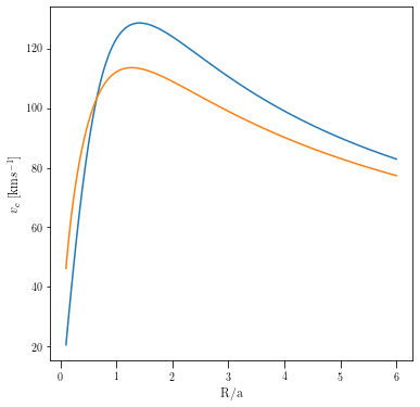
One can compute the circular velocity of the Kuzmin disk in the mid-plane, by equating the centrifugal force with the gravitational force at a given distance R from the disk.
\begin{eqnarray} v_{\rm c}(R) &=& \sqrt{R \frac{\partial \Phi_{\rm K}}{\partial R}}\,,\\ &=& \sqrt\frac{GMR^2}{(R^2+a^2)^{3/2}} \\ &=& \frac{1}{(1+a^2/R^2)^{3/4}} \sqrt\frac{GM}{R} \end{eqnarray}
[18]:
class Kuzmindisk:
    def __init__(self, mass, a):
        self.mass = mass
        self.a = a
        self.gee = 4.2994e-9

    def vcirc(self, R):
        return np.sqrt(self.gee*self.mass*R**2/(R**2+self.a**2)**(3./2.))

    def mass_within_R(self, R):
        return -self.mass*self.a*(1/(R**2+self.a**2)**(1./2.)-1/self.a)

    def vcirc_mass_within_R(self, R):
        return sqrt(self.gee*self.mass_within_R(R)/R)

# 10^11 Msun disk with radius 10 kpc
aa = Kuzmindisk(1e11, 0.010)
RR = np.logspace(-3, np.log10(0.060), 100)

ax = pl.subplot(111)
plot(RR/0.010, aa.vcirc(RR))
plot(RR/0.010, aa.vcirc_mass_within_R(RR))
ax.set_xlabel("R/a")
ax.set_ylabel(r"$v_{\rm c}$ [km$s^{-1}$]")
[18]:
Text(0, 0.5, '$v_{\\rm c}$ [km$s^{-1}$]')
Miyamoto-Nagai disk model
The density potential pair of Kuzmin can be generalized to thicker disks by considering the potential (Miyamoto and Nagai 1975)
\begin{equation} \Phi_{\rm M}(R, z) = -\frac{GM}{\sqrt{R^2+(a+\sqrt{z^2+b^2})^2}} \,. \end{equation}
Depending upon the magnitude of \(a\) compared to \(b\), one can get a spherical or a highly flattened system. One can obtain the density distribution corresponding to this potential via the Poisson equation and it turns out to be
\begin{equation} \rho_{\rm M}(R, z) = \left(\frac{b^2M}{4\pi}\right) \frac{aR^2+\left(a+3\sqrt{z^2+b^2}\right)\left(a+\sqrt{z^2+b^2}\right)^2}{\left[ R^2+\left(a+\sqrt{z^2+b^2}\right)^2\right]^{5/2}\left(z^2+b^2\right)^{3/2}} \end{equation}
General azimuthally symmetric distributions
There are different ways to approach the problem of general azimuthally symmetric distributions. One approach for obtaining potential density pairs for azimuthally symmetric distributions is by considering oblate distributions, and taking the limit where the non-equal axis becomes very thin.
Another approach is by directly performing the integral over the density distribution to get to the potential. This involves elliptical integrals.
One can also approach the problem by obtaining solutions to the Poisson equation for a thin disk away from the disk, this approach involves Bessel functions and Hankel transforms. Let us take a brief look at this approach.
Bessel function approach
For an axially symmetric system, the Poisson equation far away from the disk reduces to
\begin{eqnarray} 0 = \nabla^2\phi &=& \frac{1}{R}\frac{\partial }{\partial R} \left(R\frac{\partial \Phi}{\partial R}\right) + \frac{1}{R^2}\frac{\partial^2}{\partial \phi^2} \Phi + \frac{\partial^2 \Phi}{\partial z^2}\\ &=& \frac{1}{R}\frac{\partial }{\partial R} \left(R\frac{\partial \Phi}{\partial R}\right) + \frac{\partial^2 \Phi}{\partial z^2} \end{eqnarray}
where the second term in the first equation above for the Laplacian is zero due to axial symmetry. Given that the two terms in the following equation are independent, we can solve this equation using separation of variables. Defining \(\Phi(R, z) = P(R)Q(z)\), we obtain
\begin{equation} \frac{1}{P(R)R}\frac{d}{dR}\left( R\frac{dP}{dR}\right) = -\frac{1}{Q(z)} \frac{d^2Q}{dz^2} \end{equation}
Given that the LHS is independent of \(z\) while the RHS is independent of \(R\), the above expressions can only be equal if they were equal to a constant. We can set both equal to -\(k^2\). For the z component, we have
\begin{equation} \frac{1}{Q(z)} \frac{d^2Q}{dz^2} = k^2 \,, \end{equation}
which has the solution
\begin{equation} Q(z) = Q_0 \exp(\pm kz) \end{equation}
If \(k\) is complex, this can result in oscillatory behaviour as \(z\rightarrow \infty\). Thus physical solutions which would require \(Q\rightarrow 0\) as \(z\rightarrow \infty\), demand \(k \gt 0\), with a minus sign in the above expression for \(z\gt 0\). For \(z\lt 0\), we would require the positive sign with \(k\gt 0\).
The other equation,
\begin{equation} \frac{1}{R}\frac{d}{dR}\left( R\frac{dP}{dR}\right) = -k^2 P(R) \end{equation}
The solution to this equation is the Bessel’s function of the first kind \(J_{\rm \alpha}(kR)\), with \(\alpha=0\).
Thus,
\begin{equation} \Phi(R, z) = \exp\left(-k|z|\right) J_0(kR) \end{equation}
for positive \(k\) is a solution to the Poisson equation \(\nabla^2\Phi=0\). Now these solutions solve the Poisson equation for all \(z\neq 0\). The discontinuity at \(z=0\) helps to obtain the surface density of the disk, by performing a volume integral over a small cylinder straddling \(z=0\).
\begin{equation} \Sigma_k(R) = -\frac{k}{2\pi G} J_0(kR) \end{equation}
Given that solutions to the Poisson equation can be added up to obtain new solutions, it is clear that a givne surface density \(\Sigma(R)\) could be decomposed in to functions made of the above basis.
\begin{equation} \Sigma(R) = -\int \tilde\Sigma(k) \frac{k}{2\pi G} J_0(kR) dk\,. \end{equation}
and then use an integral over k of the Bessel functions to obtain the potential \(\Phi(R, z)\),
\begin{equation} \Phi(R, z) = \int \tilde\Sigma(k) J_0(kR)\exp(-k|z|) dk \end{equation}
Inverting the equation for \(\Sigma(R)\) gives
\begin{equation} \Sigma(k) = -2\pi G \int \Sigma(R) R J_0(kR) dR\,. \end{equation}
Substituting in the equation for the potential we finally obtain
\begin{equation} \Phi(R, z) = -2 \pi G \int \int \Sigma(R') R' J_0(kR') dR' J_0(kR)\exp(-k|z|) dk\,. \end{equation}
The circular velocity in the mid-plane can be obtained by using
\begin{equation} v_{\rm c}^2(R) = -R \left.\frac{d\Phi(R,z)}{dR}\right|_{z=0}\,. \end{equation}
The derivative \(dJ_0(x)/dx\) equals \(-J_1(x)\), which implies
\begin{equation} v_{\rm c}^2(R) = -R \int_0^\infty \tilde\Sigma(k) J_1(kR) k dk\,. \end{equation}
This equation can in principle be inverted in order to obtain \(\tilde \Sigma(k)\) and thus \(\Sigma(R)\). This route involves usage of the derivatives of \(v_{\rm c}^2(R)\) with respect to \(R\), which could potentially be obtained observationally. However the propagation of errors in the measurement of \(v_{\rm c}^2(R)\) to the derivatives of \(v_c^2(R)\) is quite cumbersome, and hence it is better to just use a model for \(\Sigma(R)\), compute \(\Sigma(k)\) and fit to \(v_{c}^2(R)\).
Vertical structure of the potential of infinitesimally thin disks
The Poisson equation in cylindrical coordinate system is
\begin{equation} \frac{\partial^2\Phi}{\partial z^2} + \frac{1}{R}\frac{\partial}{\partial R}\left[ R \frac{\partial \Phi}{\partial R}\right] = 4\pi G\rho(R, z)\,. \end{equation}
The second term on the left hand size is finite irrespective of the thickness of the disk, while the first term can grow up as we consider infinitesimally thin systems. This equation helps to approximately compute the potential of disks given their density distribution. First approximate the disk as thin, and compute the radial variation of the potential. Then we can use the equation to compute the variation of the potential in the z direction.
\begin{equation} \frac{\partial^2\Phi}{\partial z^2} = 4\pi G\rho(R, z)\,. \end{equation}