Friedmann Robertson Walker models
In this section, we will take a look at some consequences of the Friedmann Robertson Walker metric that we derived for a homogeneous and isotropic Universe.
Redshifts in an expanding Universe
Light travels on null geodesics, and they satisfy \(ds^2=0\) . Let us consider the position of our galaxy to be at the origin as a convenience. Let us look at a galaxy whose coordinates are (\(\chi, \theta, \phi\)). The light coming from this galaxy will travel along constant values of (\(\theta, \phi\)) on its path to us. Thus it should satisfy
\(ds^2=0=-c^2 dt^2 + a^2(t) d\chi^2\)
which implies that
\begin{equation} \int_{t_e}^{t_r} \frac{c dt}{a(t)} = -\int_{0}^{\chi} d\chi \end{equation}
where \(t_e\) denotes the time of emission, \(t_r\) denotes the time of receipt of the photon. Now let us consider the emission and reception of a consecutive crest of the light wave. Let us suppose this second crest gets emitted at \(t_e + \delta t_e\), and will be received \(t_r + \delta t_r\). This implies that for this second crest,
\begin{equation} \int_{t_e+\delta t_r}^{t_r + \delta t_r} \frac{c dt}{a(t)} = -\int_{0}^{\chi} d\chi \end{equation}
Subtracting the above equations we get
\begin{equation} \frac{c \delta t_e}{a(t_e)} - \frac{c \delta t_r}{a(t_r)}= 0 \end{equation}
Given that \(\lambda_e = c\delta t_e\) and \(\lambda_r = c\delta t_r\), are the wavelengths of the emitted and received light, we obtain
\begin{equation} \frac{\lambda_r}{\lambda_e} = 1+z = \frac{a(t_r)}{a(t_e)} \end{equation}
This implies that the wavelength of light changes as it travels in a Universe with varying scale factor. If \(a(t)\) is an increasing function of time then this implies that the wavelength of the received light will be redshifted compared to when the light was emitted.
Expansion of the Universe (Hubble-Lemaitre’s law)
The FRW metric implies that the physical distances in the Universe scale with the scale factor. We can define mean motion coordinates which move together in a concerted manner due to the change in scale factor. Such coordinates are called comoving coordinates. The physical distance between any two locations at a given point of time is thus given by \(R_{\rm phys} = a(t) R_{\rm com}\) . The velocity between any two objects is then given by the rate of change of the physical distance
\begin{eqnarray} v = \frac{d R_{\rm phys}}{dt} &=& \frac{d \left[ a(t) R_{\rm com} \right]}{dt} \\ &=& \frac{da}{dt} R_{\rm com} + a(t) \frac{d R_{\rm com}}{dt} \\ &=& \frac{\dot{a}}{a} R_{\rm phys} + a(t) \frac{d R_{\rm com}}{dt} \end{eqnarray}
For fundamental observers at fixed locations in the comoving coordinates, the second term would be zero. This gives
\begin{equation} v = \left[\frac{\dot{a}}{a}\right] R_{\rm phys} \end{equation}
This shows that the velocities should be proportional to the physical distance of galaxies. The constant of proportionality \(\dot{a}/a\) is called the Hubble-Lemaitre parameter. Note that \(\dot{a}/a\) is a function of time, the value at \(t={\rm today}\) is called the Hubble-Lemaitre constant.
In reality galaxies will not necessarily sit still in comoving coordinates due to forces from other objects nearby. These velocities are called peculiar velocities and are a result of the small scale inhomogenieties in the Universe.
The measurement of the Hubble Lemaitre constant is one of the biggest scientific inquiries currently. The value that Hubble derived in the 1920s was about \(500\) \({\rm km/s/Mpc}\). It was marred by observational issues. The current accepted value for the Hubble constant ranges from \(67\) to \(74\) \({\rm km/s/Mpc}\).
The units of the Hubble-Lemaitre constant are the inverse of the timescale. Thus the Hubble-Lemaitre constant sets a time scale in the Universe. The value of \(1/H_0\) sets the order of magnitude for the timescale for the Universe. With the value of about \(70\) \({\rm km/s/Mpc}\), you get a value which is close to \(1.46\times10^{10}\) years.
Distances in the Universe
Angular size of a distant object of known physical size
Consider the angle subtended at the observer by a known object of physical size \(R_{\rm phys}\) at a coordinate distance \(\chi\). Let us assume that the two ends of the object are aligned at constant angle \(\phi\). Thus in the metric we have \(dt=0\), \(d\chi=0\) and \(d\phi=0\). The metric is then given by
\begin{equation} ds^2 = a^2(t) f^2(\chi) d\theta^2 \end{equation}
The physical size of the object \(R_{\rm phys}=a(t) f(\chi) \Delta \theta\). We can define a distance based on the angular size subtended by such an object as the angular diameter distance.
\begin{equation} D_{\rm ang} = \frac{R_{\rm phys}}{\Delta\theta} = a(t) f(\chi) = \frac{f(\chi)}{(1+z)} \end{equation}
Exercise:
Can you compute the physical area of the sphere at coordinate \(\chi\) away from the observer situated at the origin?
Can you define the two dimensional analog of this problem on the surface of a sphere?
Can you compute the comoving coordinate volume of a sphere centered at the origin with radius given by the coordinate \(\chi\)?
Flux received from a distant source
Let us now consider the flux received from a distant source in the Universe, which has an intrinsic bolometric luminosity \(L\) (i.e., integrated over all wavelengths). We can write the luminosity emitted per unit wavelength as
\begin{equation} dL = L I(\lambda) d\lambda \end{equation}
where
\begin{equation} \int I(\lambda) d\lambda = 1 \end{equation}
Remember luminosity is the energy emitted per unit time. The number of photons emitted per unit wavelength \(\lambda_e\) in a time \(\delta t_e\) are given by
\begin{equation} dN(\lambda_e) = dL \delta t_e \frac{\lambda_e}{hc} = L \frac{\lambda_e}{hc} I(\lambda_e) d\lambda_e \delta t_e \end{equation}
The light emitted from the source will reach a sphere at coordinate \(\chi\) after time \(t\). The spacetime metric for constant time and constant \(\chi\) value is given by \(ds^2 = a^2(t) f^2(\chi) [d\theta^2 + \sin^2\theta d\phi^2]\) which is the line element on the surface of a sphere with radius \(a^2(t) f^2(\chi)\). The surface area of this sphere is given by
\begin{equation} \int a^2(t_r) f^2(\chi) d\cos\theta d\phi = 4 \pi a^2(t_r) f^2(\chi) \end{equation}
We observe these photons today, thus \(a^2(t_r)=1\) by definition of the coordinate system to define lengths. The number of photons received per unit wavelength \(\lambda_r\) over the entire surface of the sphere is given by
\begin{equation} dN_r(\lambda_r) = dN_e\left( \frac{\lambda_r}{(1+z)}\right) = L \frac{\lambda_r}{(1+z)hc} I \left( \frac{\lambda_r}{1+z} \right) \frac{d\lambda_r}{(1+z)} \delta t_e \end{equation}
Here we have used the fact that the wavelength changes as time goes on in the Universe. Now these photons will be received in an interval of time \(\delta t_r\) as we saw in the derivation in the first section. Thus the amount of energy that passes through the sphere in a unit time interval is given by
\begin{equation} \frac{dN_r(\lambda_r)}{\delta t_r} \frac{hc}{\lambda_r} = L \frac{1}{(1+z)} I \left( \frac{\lambda_r}{1+z} \right) \frac{d\lambda_r}{(1+z)} \frac{\delta t_e}{\delta t_r} \end{equation}
The flux \(F(\lambda_r) d\lambda_r\) is the amount of energy received per unit time per unit area perpendicular to the line of sight to the source. Thus \(F(\lambda_r) d\lambda_r\) should be equal to
\begin{eqnarray} F(\lambda_r) d\lambda_r &=& \frac{dN_r(\lambda_r)}{\delta t_r} \frac{hc}{\lambda_r} \frac{1}{4\pi f^2(\chi) a^2(t_r)} \\ &=& \frac{L}{(1+z)} I \left( \frac{\lambda_r}{1+z} \right) \frac{d\lambda_r}{(1+z)} \frac{\delta t_e}{\delta t_r} \frac{1}{4\pi f^2(\chi) } \\ &=& \frac{L}{(1+z)^2} I \left( \frac{\lambda_r}{1+z} \right) d\lambda_r \frac{\delta t_e}{\delta t_r} \frac{1}{4\pi f^2(\chi) } \\ &=& \frac{L}{(1+z)^3} I \left( \frac{\lambda_r}{1+z} \right) d\lambda_r \frac{1}{4\pi f^2(\chi)} \end{eqnarray}
The total bolometric flux is given by the integral over all wavelengths and therefore
\begin{equation} F_{\rm bol} = \int F(\lambda_r) d\lambda_r = \frac{L_{\rm bol}}{(1+z)^2 4\pi f^2(\chi)} = \frac{L_{\rm bol}}{4\pi D_{\rm lum}^2(\chi)} \end{equation}
This can be intuitively understood as all photons lose energy and arrive at stretched out intervals as the Universe expands. The luminosity distance defined by the last equality is thus given by \begin{equation} D_{\rm lum}(\chi) = (1+z) f(\chi) \end{equation}
Dynamics of the Friedmann Robertson Walker metric
Now let us try to understand how the scale factor of the Universe changes as a function of time. The equations of General Relativity govern the dynamics in the Universe. \begin{equation} G_{\mu\nu} = \frac{8 \pi G}{c^4} T_{\mu\nu} \end{equation} where \(G_{\mu\nu}\) is the Einstein tensor, and \(T_{\mu\nu}\) is the energy momentum tensor of the Universe. The left hand side of the equation concerns the metric and its derivatives. So this can be computed based on the metric components that we haver derived heuristically above.
We consider the coordinates to be \(ct, \chi, \theta, \phi\) as \(0, 1, 2, 3\): \begin{equation} g_{\mu \nu} = \begin{pmatrix} -1 & 0 & 0 & 0 \\ 0 & a^2(t) & 0 & 0 \\ 0 & 0 & a^2(t)f^2(\chi) & 0 \\ 0 & 0 & 0 & a^2(t)f^2(\chi)\sin^2(\theta) \end{pmatrix} \end{equation}
One can compute the Christoffel symbols for this metric using their definition
\begin{equation} \Gamma^i_{kl} = \frac{1}{2}g^{im}\left[ g_{mk,l} + g_{ml,k} - g_{kl,m} \right] \end{equation}
Exercise:
Show that \(\Gamma^{0}_{\mu\nu} = \frac{1}{2}g_{\mu\nu}\).
Then we can use these Christoffel symbols derived from the metric to compute the Riemann tensor
\begin{equation} R^{\rho}{}_{\sigma\mu\nu} = \partial_\mu \Gamma^{\rho}_{\nu\sigma} - \partial_{\nu} \Gamma^\rho_{\mu\sigma} + \Gamma^\rho_{\mu\lambda} \Gamma^\lambda_{\nu\sigma} - \Gamma^\rho_{\nu\lambda} \Gamma^\lambda_{\mu\sigma} \end{equation}
The Riemann tensor can then be contracted to obtain the Ricci tensor by taking a trace
\begin{equation} R_{\mu\nu} = R^\lambda{}_{\mu\lambda\nu} \end{equation}
and the Ricci scalar to obtain
\begin{equation} R = g^{\mu\nu}R_{\mu\nu} \end{equation}
These components can be finally combined to obtain the Einstein tensor
\begin{equation} G_{\mu\nu} = R_{\mu\nu} - \frac{1}{2}R g_{\mu\nu} \end{equation}
All of these involve tedious but straightforward mathematics and we will just quote the final results here:
\begin{eqnarray} G_{00} = 3 \left(\frac{\dot{a}}{a} \right)^2 + 3\frac{kc^2}{a^2} \\ G_{ij} = - \left( 2\frac{\ddot{a}}{a} + \left[\frac{\dot{a}}{a}\right]^2 + \frac{k c^2}{a^2} \right) a^2 \gamma_{ij}\,, \end{eqnarray}
where \(\gamma_{ij}\) is the metric of the homoegenous and isotropic 3-space, i.e., \(dl^2 = \gamma_{ij}dx^{i}dx^{j}\). The other components are equal to zero. In what follows, I will show a useful way to compute these tensors in python. We will use the packages einsteinpy and sympy to carry out these tedious mathematical calculations. In your sciserver environment, you could install these packages by typing %pip install --user einsteinpy and restarting the jupyter kernel
by clicking Kernel and then Restart.
[6]:
# Import important packages

import sympy
from einsteinpy.symbolic import MetricTensor, ChristoffelSymbols, RiemannCurvatureTensor, RicciTensor, RicciScalar, EinsteinTensor
from sympy import Function, simplify

# Enable the best printing solution
sympy.init_printing()
[16]:
# Define symbols

def get_metric(univ_type):
    syms = sympy.symbols("t chi theta phi")
    t, chi, theta, phi = syms
    a, R, c = sympy.symbols("a R c")

    # Initialize a 2d 4x4 array
    list2d = [[0 for i in range(4)] for i in range(4)]

    # Define the function f depending upon the type of the Universe
    def f(x, universe):
        if universe=="flat":
            return x
        if universe=="closed":
            return sympy.sin(x)
        if universe=="open":
            return sympy.sinh(x)

    # Set the diagonal elements to be g_{\mu\nu}
    list2d[0][0] = -1
    list2d[1][1] = Function(a)(t)**2
    list2d[2][2] = Function(a)(t)**2*(R*f(chi/R, univ_type))**2
    list2d[3][3] = Function(a)(t)**2* (R*f(chi/R, univ_type))**2 * (sympy.sin(theta) ** 2)

    # Define the metric
    frw = MetricTensor(list2d, syms)

    # Visualize the metric
    frw.tensor()

    return frw
[17]:
open_metric = get_metric("open")
closed_metric = get_metric("closed")
flat_metric = get_metric("flat")
[18]:
open_metric.tensor()
[18]:
[19]:
simplify(EinsteinTensor.from_metric(open_metric).tensor()[1,1]/open_metric.tensor()[1, 1])
[19]:
[20]:
simplify(EinsteinTensor.from_metric(flat_metric).tensor()[1,1]/flat_metric.tensor()[1, 1])
[20]:
[21]:
simplify(EinsteinTensor.from_metric(closed_metric).tensor()[1,1]/closed_metric.tensor()[1, 1])
[21]:
[22]:
simplify(EinsteinTensor.from_metric(closed_metric).tensor()[0,0])
[22]:
The energy momentum tensor
The energy momentum tensor \(T_{\mu\nu}\) is the flux of the 4-momentum \(p_{\mu}\). In a homogeneous and isotropic Universe it must have only a diagonal form, with the space components all being equal. In the lecture course on GR, you have encountered the energy momentum tensor of ideal fluid, which is exactly what we will use for the energy momentum tensor in the Einstein field equations for the Universe. The ideal fluid is described by its density \(\rho\) and pressure \(p\). The energy momentum tensor is given by
\begin{equation} T_{\mu \nu} = (\rho c^2 + p) u_{\mu} u_{\nu} + p c^2 g_{\mu\nu} \end{equation}
For fundamental observer which move with the mean motion of the Universe, \(u_{\mu}=[c, 0, 0, 0]\), because the three spatial coordinates do not change with time, and the derivative of the first coordinate \(ct\) with respect to proper time is just \(c\). For the zero zero component,
\begin{eqnarray} T_{00} &=& \rho(t) c^4 \\ T_{ij} &=& p(t) c^2 a^2(t) \gamma_{ij} \end{eqnarray}
Equating the \(00\) component of the Einstein’s field equations, we get the first of the Friedmann equations, \begin{equation} \left[ \left(\frac{\dot{a}}{a}\right)^2 + \frac{kc^2}{a^2} \right] = \frac{8\pi G \rho}{3} \end{equation}
and the second equation corresponds to the \(ij\) components \begin{equation} - \left[ \frac{2\ddot{a}}{a} + \left(\frac{\dot{a}}{a}\right)^2 + \frac{k c^2}{a^2} \right] = 8 \pi G \frac{p}{c^2} \end{equation}
The above two equation can be combined to obtain
\begin{equation} \frac{\ddot{a}}{a} = - \frac{4\pi G}{3} \left(\rho + \frac{3 p}{c^2}\right) \end{equation}
This shows that for energy density in the Universe with a non-negative pressure, the scale factor \(a(t)\) cannot have a positive acceleration.
The two equations given above also imply the following intuitive conservation equation if you multiply the first equation by \(a^3\) and then differentiating and getting rid of the second derivative term using the second equation:
\begin{equation} \frac{d}{dt}\left[ a^3 \rho c^2 \right] + p \frac{d}{dt}\left[ a^3 \right] = 0 \end{equation}
Exercise:
Prove the equality given above using the Friedmann equations.
Show that this equality also implies \begin{equation} \frac{d\rho}{dt} + 3 \frac{\dot{a}}{a} \left(\rho + \frac{p}{c^2}\right) = 0 \end{equation}
Let us take a look at the first Friedmann equation to compute the evolution of the scale factor of the Universe.
\begin{equation} \left[ \left(\frac{\dot{a}}{a}\right)^2 + \frac{kc^2}{a^2} \right] = \frac{8\pi G \rho}{3} \end{equation}
What are the initial conditions for this problem. Since the scale factor is a growth factor we are free to choose the normalization. Let us work with the condition that \(a(t)=1\) today. The factor \({\dot{a}}/{a}\) is nothing but the Hubble Lemaitre constant today whose value can be measured with observations. Thus the value of Hubble Lemaitre constant \(H_0\) is our second initial condition. This along with the behaviour of energy density with \(a\) should allow us to integrate the above equation.
Before we solve the Friedmann equation, notice that for the Universe to be spatially flat, the density of the Universe today should be equal to a very special value \begin{equation} \rho_{\rm crit} = \frac{3H_0^2}{8\pi G} \end{equation}
\begin{eqnarray} \left(\frac{\dot{a}}{a}\right)^2 &=& H_0^2 \left[ \frac{\rho}{\rho_{\rm crit}} - \frac{kc^2}{a^2H_0^2} \right] \end{eqnarray} Substituting \(\dot{a}/a = H_0\) today, we find that. \begin{eqnarray} 1 &=& \left[ \frac{\rho_0}{\rho_{\rm crit}} - \frac{kc^2}{H_0^2} \right] \\ -\frac{kc^2}{H_0^2} &=& \left[ 1 - \frac{\rho_0}{\rho_{\rm crit}} \right] : = \Omega_{\rm k, 0} \end{eqnarray} If the Universe is denser than \(\rho_{\rm crit}\) today, then it has a closed geometry \(k>0\), while a Universe which is less dense than the critical density will have an open geometry with \(k<0\). Thus we can simplify the Friedmann equation to
\begin{eqnarray} \left(\frac{\dot{a}}{a}\right)^2 &=& H_0^2 \left[ \frac{\rho}{\rho_{\rm crit}} + \frac{\Omega_{\rm k, 0}}{a^2} \right] \end{eqnarray}
Now we need to figure out how the density of the Universe changes as a function of time. Let us consider a few cases to understand the evolution of these components in a non-static Universe. Let us first consider just matter. For matter the pressure comes from velocities. However given that the velocities of matter are non-relativistic, the pressure is negligible compared to the energy density. Thus for matter, we have \(p << \rho c^2\), and it can be ignored. The equation of energy conservation then implies
\begin{equation} \frac{d}{dt}\left[ a^3 \rho c^2 \right] = 0 \end{equation}
Thus the matter density \(\rho_{\rm m} \propto a^{-3}\), the density decreases if the Universe expands, and increases if the Universe contracts. This is consistent with the increase in the total volume of the Universe \(\propto a^3\) due to the increase in scale factor, and thus the density decreases by the same factor \(a^3\) if there is conservation of matter in a comoving volume.
What about another form of energy density in the Universe, that of radiation. One can show that the photon energy density is related to the pressure such that
\begin{equation} p = \frac{1}{3} \rho c^2 \end{equation}
Plugging this into the pressure density equation, we find \begin{equation} \rho_{\rm rad} \propto a^{-4} \end{equation}
The energy density of radiation changes due to the change in volume as well as the change in energy that a photon undergoes when the Universe expands or contracts.
Exercise:
Find how the density of an ideal fluid with pressure \(p =w \rho c^2\) evolves in a non-static Universe as a function of the scale factor.
The real Universe can have fluids of different kinds all together thus the combined Friedmann equation looks like
\begin{eqnarray} \left(\frac{\dot{a}}{a}\right)^2 &=& H_0^2 \left[ \frac{\rho_m}{\rho_{\rm crit}} + \frac{\rho_{\rm rad}}{\rho_{\rm crit}} + \frac{\rho_{\rm w}}{\rho_{\rm crit}} + \frac{\Omega_k}{a^2} \right] = H_0^2 E^2(a) \end{eqnarray}
Analogous to \(\Omega_{\rm k}\) we can define \(\Omega_{\rm x, 0} = \rho_{\rm x, 0}/\rho_{\rm crit}\) which finally reduces the equation to a much more manageable form \begin{eqnarray} \left(\frac{\dot{a}}{a}\right)^2 &=& H_0^2 \left[ \Omega_{\rm m, 0} a^{-3} + \Omega_{\rm rad, 0} a^{-4} + \Omega_{\rm w, 0}a ^{-3(1+w)} + \Omega_k a^{-2} \right] = H_0^2 E^2(a) \end{eqnarray} where \(\Omega_{\rm k} = 1 - \Omega_{\rm m} - \Omega_{\rm rad} - \Omega_{\rm w, 0}\). Current observations indicate that a special fluid called dark energy with an equation of state \(w=-1\) is required to be present in the Universe. Thus we will assume that the Universe has these combinations of fluid (matter, radiation and \(\Lambda\)).
Matter dominated Universe
First let us consider a Universe just made up of matter. In this case the Friedmann equation is very simple \begin{eqnarray} \left(\frac{\dot{a}}{a}\right) &=& H_0 \left[\Omega_{\rm m, 0}a^{-3} + (1-\Omega_{\rm m,0}) a^{-2} \right]^{1/2} \end{eqnarray} In such a Universe, we can obtain \(\dot{a}=0\), if and only if \begin{equation} \Omega_{\rm m, 0}a^{-3} + (1-\Omega_{\rm m,0}) a^{-2} = 0 \end{equation} which gives a special epoch \begin{equation} a = \frac{\Omega_{\rm m, 0}}{(\Omega_{\rm m,0}-1)} \end{equation} Notice that this has a non-negative scale factor only if \(\Omega_{\rm m,0}>1\). Thus if the Universe has \(\Omega_{\rm m}>1\) which corresponds to \(\Omega_{\rm k}<0\), the scale factor has a maximum. Given that the Universe is expanding today it means that the Universe will stop its expansion at a finite future, and given that the value of \(\ddot{a}<0\), such a Universe will start contracting.
For \(\Omega_{\rm m, 0}=1\), the Universe keeps on increasing at an ever slow pace and only asymptotically reaches \(\dot{a}=0\), while for a \(\Omega_{\rm m,0}<1\), the Universe keeps on expanding but never reaches a scale factor where the expansion halts.
Let us consider one of these special cases: \(\Omega_{\rm m,0}=1\). In this case, we obtain \begin{eqnarray} \left(\frac{\dot{a}}{a}\right) &=& H_0 a^{-3/2} \\ \int_{a}^{1} a^{1/2} da &=& \int_{t}^{t_0} H_0 dt \\ \left.\frac{2a^{3/2}}{3}\right|_{a}^{1} &=& H_0(t_0-t) \\ a(t) &=& \left[1 - \frac{3}{2}H_0 (t_0-t)\right]^{2/3} \end{eqnarray} In this model the current age of the Universe \(t_0\) is related to the time at which \(a=0\) as \begin{eqnarray} t_0-t = \frac{2}{3H_0} \end{eqnarray}
Radiation dominated Universe
In the early Universe when it was small, radiation is expected to dominate the energy density of the Universe as it increases quicker than \(\rho_{\rm m}\) as \(a\rightarrow 0\). In this case the Friedmann equation looks like \begin{eqnarray} \left(\frac{\dot{a}}{a}\right) &=& H_0 \Omega_{r, 0} a^{-2} \\ \int a da &=& \int H_0 \Omega_{r, 0} dt \\ \frac{a^2}{2} &=& H_0 \Omega_{r, 0} t \\ a(t) &=& [2 H_0 \Omega_{r, 0} t]^{1/2} \end{eqnarray}
Lambda dominated Universe
On the other hand, when \(a>>1\), we expect the Universe to be dominated by \(\Omega_{\rm \Lambda}\). The Friedmann equation for that case looks like \begin{eqnarray} \left(\frac{\dot{a}}{a}\right) &=& H_0 \Omega_{\Lambda, 0} \\ \end{eqnarray} and we obtain \begin{eqnarray} a(t) = \exp\left[ H_0 \Omega_{\Lambda, 0} (t-t_0) \right] \\ \end{eqnarray} and the Universe will reach a state of exponential expansion.
From all these simple homogeneous and isotropic models, we can work out the expansion history of the Universe, its age, and its fate by making some simple measurements of the energy density of various constituents in the Universe and the Hubble Lemaitre constant which measures the rate of expansion of the Universe today! A number of cosmology experiments use these simple equations to relate scale factor and time to help us understand the history and fate of the Universe.
Horizons in the Universe
Because light travels at a finite speed in the Universe, it can only travel a finite distance from a source given the age of the Universe today. Let us compute what is the comoving distance light would have travelled from \(a=0\) to today \(a=1\).
\begin{eqnarray} \chi_{\rm horizon} &=& \int_0^{1} \frac{cdt}{a(t)} \\ &=& \int_0^{1} \frac{cda}{\dot{a}a(t)} \\ &=& \int_0^1 \frac{cda}{\frac{\dot{a}}{a} a^2(t)} \\ &=& \int_0^1 \frac{cda}{H_0 E(a) a^2(t)} \end{eqnarray}
This is a finite quantity. Given causality, anything in the Universe can not be affected by object beyond its horizon.
[165]:
import numpy as np
from scipy.integrate import quad
from scipy import optimize


class cosmology:

    def __init__(self, Omega_m, Omega_r, Omega_l, H0):
        self.Omega_m = Omega_m
        self.Omega_r = Omega_r
        self.Omega_l = Omega_l
        self.H0 = H0

        # Define the curvature based on the Friedmann equation evaluated at t=today.
        self.Omega_k = 1 - Omega_m - Omega_r - Omega_l

        self.a_max = self.max_scale_factor()
        print(self.a_max, "Maximum scale factor")

    def zofa(self, a):
        return 1./a - 1.

    def aofz(self, z):
        return 1/(1.+z)

    # Define the RHS of the Friedmann equation
    def Esqofa(self, a):
        return (self.Omega_m*a**-3 + self.Omega_r*a**-4 + self.Omega_l + self.Omega_k*a**-2 )

    # Define derivative of the RHS of the Friedmann equation
    def Esqprimeofa(self, a):
        return (-3.*self.Omega_m*a**-4 - 4.*self.Omega_r*a**-5 - 2.*self.Omega_k*a**-3 )

    # Define the RHS of the Friedmann equation
    def Eofa(self, a):
        return (self.Omega_m*a**-3 + self.Omega_r*a**-4 + self.Omega_l + self.Omega_k*a**-2 )**0.5

    # Define derivative of the RHS of the Friedmann equation
    def Eprimeofa(self, a):
        return (-3*self.Omega_m*a**-4 - 4*self.Omega_r*a**-5 - 2*self.Omega_k*a**-3 )/(self.Omega_m*a**-3 + self.Omega_r*a**-4 + self.Omega_l + self.Omega_k*a**-2 )**0.5


    # Define the time given a scale factor (time will be returned in units of 1/H0)
    def compute_time_given_scale(self, a, contracting=False):

        # Integrate the function \int da/a/E(a) = \int d(t/(1/H0))
        def integrand(ap):
            return 1/ap/self.Eofa(ap)

        if a>self.a_max:
            return np.nan

        answer = 0
        if contracting:
            exp_soln, error = quad(integrand, 1, self.a_max)
            cont_soln, error2 = quad(integrand, self.a_max, a)
            answer = exp_soln - cont_soln
        else:
            answer, error = quad(integrand, 1, a)

        return answer

    # Compute maximum scale factor if the Universe is closed based on the zero of Eofa
    def max_scale_factor(self):
        if self.Omega_k>=0:
            return np.inf

        # Compute the zero of the expansion factor
        sol = optimize.root_scalar(self.Esqofa, x0=1.0, fprime=self.Esqprimeofa, method='newton')

        if sol.flag == "convergence error":
            sol.root = np.inf

        return sol.root


    # Exercise:
    # Write code to compute coordinate distance $\chi$ as a function of the scale factor
    # Integrand is: \int c dt/a(t) = \int dchi
    # Forget about the contracting case for now.

    # Write code to compute angular diameter distance as a function of the scale factor
    # f(chi) * a(t)

    # Write code to compute the luminosity distance as a function of the scale factor
    # f(chi) / a(t)

    # Write code to compute the comoving distance travelled by light from a given scale factor to today
    # Integrand is: \int c dt/a(t) = \int c/H0 da/E(a)/a^2(t)
[166]:
flat_c = cosmology(1.0, 0.0, 0.0, 100.0)
open_c = cosmology(0.1, 0.0, 0.0, 100.0)
closed_c = cosmology(3.0, 0.0, 0.0, 100.0)
inf Maximum scale factor
inf Maximum scale factor
1.4999999999999998 Maximum scale factor
[167]:
# Compute scale factor versus time
scale_arr = np.linspace(1e-2, 3., 10000)
print(scale_arr)

time_arr_flat = scale_arr*0.0
time_arr_closed = scale_arr*0.0
time_arr_closed_cont = scale_arr*0.0
time_arr_open = scale_arr*0.0
for ii in range(scale_arr.size):
    time_arr_flat[ii] = flat_c.compute_time_given_scale(scale_arr[ii])
    time_arr_closed[ii] = closed_c.compute_time_given_scale(scale_arr[ii])
    time_arr_closed_cont[ii] = closed_c.compute_time_given_scale(scale_arr[ii], contracting=True)
    time_arr_open[ii] = open_c.compute_time_given_scale(scale_arr[ii])
[0.01 0.01029903 0.01059806 ... 2.99940194 2.99970097 3. ]
[168]:
import pylab as pl
%pylab inline

conf = %config InlineBackend.rc
conf["figure.figsize"] = (6, 6)
conf['savefig.dpi']=100
conf['font.serif'] = "Computer Modern"
conf['font.sans-serif'] = "Computer Modern"
conf['text.usetex']=True

width = 600
%config InlineBackend.rc
%pylab inline
Populating the interactive namespace from numpy and matplotlib
Populating the interactive namespace from numpy and matplotlib
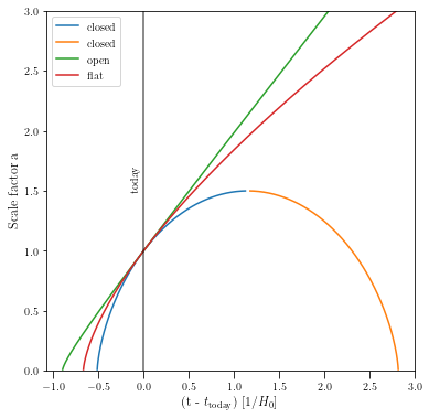
[169]:
ax = pl.subplot(111)

idx = ~(time_arr_closed==0)
ax.plot(time_arr_closed[idx], scale_arr[idx], label="closed")
ax.plot(time_arr_closed_cont[idx], scale_arr[idx], label="closed")
ax.plot(time_arr_open, scale_arr, label="open")
ax.plot(time_arr_flat, scale_arr, label="flat")
ax.set_xlabel(r"(t - $t_{\rm today})$ [1/$H_0$]")
ax.set_ylabel("Scale factor a")
ax.axvline(0.0, color="k", alpha=0.6)
ax.legend()
ax.set_ylim(0.0, 3.0)
ax.text(-0.15, 1.5, "today", rotation=90)
[169]:
Text(-0.15, 1.5, 'today')
Exercise:
Complete the simple python code above to figure out how the luminosity distance, and the angular diameter distance change as a function of the scale factor.
Make plots of these distances as a function of the scale factor.
Use the above code to see how the scale factor of the Universe changes as a function of time for a Universe with \(\Omega_{\rm m}=0.3, \Omega_{\rm r}=0.0\) and \(\Omega_{\Lambda}=0.7\).
According to the cosmological observations today, we have \(\Omega_{\rm m}=0.315\), \(\Omega_{\rm \Lambda}=0.685\), \(\Omega_{r}\sim 10^{-4}\). Given that the density of these components are a function of the scale factor, the energy densities will change. Even though the radiation energy density is extremely small today, at early times when the scale factor was small, the constituents of the Universe will be entirely dominated by radiation. Thus the behaviour of the scale factor at different times depends upon the constituents.
Exercise:
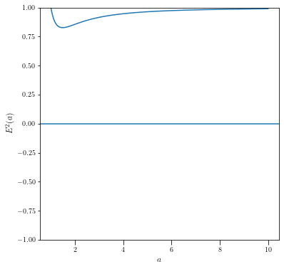
Some questions to ponder:
Does a closed Universe always mean that it will undergo a big crunch? Does a Universe with a \(\Lambda\) always mean that it will expand exponentially?
[162]:
ax = pl.subplot(111)

closed_c = cosmology(1.0, 0.1, 1.0, 100.0)

a = np.linspace(1.0, 10, 100000)
eofa = closed_c.Esqofa(a)

ax.plot(a, eofa)
ax.set_ylim(-1, 1)
ax.axhline(0)
ax.set_xlabel("$a$")
ax.set_ylabel("$E^2(a)$")
[162]:
Text(0, 0.5, '$E^2(a)$')