[1]:
from IPython.display import YouTubeVideo
The early Universe
According to the observations, the Universe is expanding today. Extrapolating backwards, this implies that the scale factor of the Universe must be quite small in the past. The radiation energy density scales as \(\rho_{\rm rad} \propto a^{-4}\). It must be the dominating source of energy density in the Early Universe, dominating over matter, \(\Lambda\) as well as the curvature. During this radiation dominated era, the temperature of the Universe would be determined by the properties of radiation. Assuming a black body nature for this radiation with temperature \(T\), and assuming that physical constants of the Universe such as the radiation constant do not depend upon time, \(\rho_{\rm rad} = 4\sigma/c T^4\), where \(\sigma\) is the Boltzmann constant. Combining the behaviour of the radiation energy density with the scale factor and its behaviour with the temperature, we obtain the relation between temperature and the scale factor, \(T \propto a^{-1}\).
The temperature of the Universe is thus inversely proportional to the scale factor, which implies that the Universe had a higher temperature at earlier epochs. Given that in the radiation dominated era, \(a \propto t^{1/2}\) where \(t\) is the time, we obtain a relation between temperature and time \(T \propto t^{-1/2}\).
Exercise:
Show that: \begin{equation} T \sim 1.5 \times 10^{10} \left[\frac{t}{\rm second}\right]^{-1/2} \end{equation} where \(t=0\) is defined to be the time when the scale factor \(a(t) = 0\).
In the earliest time in the Universe, when the temperature was of the order of \(10^{16} {\rm K} \sim 1 {\rm TeV}\), the Universe was full of elementary particles in the standard model, all in thermal equilibrium because of the high rate of interactions. The particle production and annihilation processes operate in equilibrium to keep a steady state abundance (\(na^3\)) of these particles. However as the temperature of the Universe fell due to the expansion, the production rate is not able to keep up with the annihilation rate. These changes typically happen at a temperature corresponding to the rest mass of the particles \(mc^2 \sim k_{\rm B}T\). The top quark (\(m \sim 173.07\) GeV/\(c^2\)) started to annihilate with its antiparticle at around \(t \sim 10^{-11}-10^{-12}s\). Given the mass hierarchy in the standard model, all the particle species annihilate one after the other (muons), leaving a trace amount of protons, neutrons, electrons and neutrinos. The reason why antimatter and matter had a small asymmetry (the baryon asymmetry problem) is a topic of intense research which we will not get into.
Let us consider the epoch in the Universe when it was hot enough to have free neutrons and protons around, alongwith radiation. These protons and neutrons would eventually get together to form heavier nuclei. The hot radiation prevents the formation of nuclei, however the Universe cools down as it expands, and then it becomes possible for the heavy nuclei to form. The radiation from the Universe’s hot past, would have expanded by now and cooled down, but should still be visible. In 1965, the discovery of the cosmic microwave background radiation by Arnos Penzias and Robert Wilson, which follows the blackbody curve has bolstered the idea of this hot and dense past of the Universe which was in thermodynamic equilibrium.
The different constituents of the Universe interact with each other and radiation via their standard model interactions. If we assume that thermal equilibrium holds, we can write down the distribution functions for any particular species. The distribution function gives the number of particles which have a momentum \(|\vec{p}| \pm d{p}/2\). For a species X in thermal equlibirum, the distribution function is given by
\begin{equation} f_{\rm X}(|\vec{p}|) = \frac{g_{\rm X}}{2\pi^2 \hslash^3} p^2 \left[ \exp\left( \frac{E_{\rm X}-\mu_{\rm X}}{k_{\rm B}T}\right) \pm 1 \right]^{-1} \end{equation}
where the energy \(E_{\rm X} = \sqrt{ p^2c^2 + m_{\rm X}^2c^4}\), \(\mu_{\rm X}\) is the chemical potential of a species, \(g_{\rm X}\) the number of degenerate states at a given energy level, and \(k_{\rm B}\) is the Boltzmann’s constant. The choice of the sign depends upon the nature of the species, the \(-\) sign corresponds to bosons, while the \(+\) sign corresponds to fermions.
The chemical potential for photons is zero (as they can be added or subtracted) without any change to the free energy. The chemical potentials of pairs of particles and antiparticles are opposite in sign to each other, as they can annihilate and create photons. The chemical potentials are dependent upon the number densities of these particles. The ratio of the number density of baryons to photons is quite small today (\(\sim 10^{-8}-10^{-9}\)). This ratio is constant as both the number densities fall as \(a^{-3}\). The lepton density is also small, and so all the chemical potentials can be assumed to be close to zero and negligible.
One can compute the number density, energy density, pressure and entropy density of particles in thermal equilibrium using the equations
\begin{eqnarray} n_{\rm X} &=& \int_0^{\infty} f_{\rm X} dp = \int_0^{\infty} \frac{g_{\rm X}}{2\pi^2 \hslash^3} p^2 \left[ \exp\left( \frac{E_{\rm X}}{k_{\rm B}T}\right) \pm 1 \right]^{-1} dp \\ \rho_{\rm x} c^2 =\epsilon_{\rm X} &=& \int_0^{\infty} E_{\rm X}(p) f_{\rm X} dp = \int_0^{\infty} (p_{\rm X}^2c^2+m_{\rm X}^2c^4)^{1/2} \frac{g_{\rm X}}{2\pi^2 \hslash^3} p^2 \left[ \exp\left( \frac{E_{\rm X}}{k_{\rm B}T}\right) \pm 1 \right]^{-1} dp \\ P_{\rm X} &=& \int_0^{\infty} \frac{p^2 c^2}{3 E_{\rm X}} f_{\rm X} dp = \int_0^{\infty} \frac{p^2 c^2}{3 (p^2c^2+m_{\rm X}^2c^4)^{1/2} } \frac{g_{\rm X}}{2\pi^2 \hslash^3} p^2 \left[ \exp\left( \frac{E_{\rm X}}{k_{\rm B}T}\right) \pm 1 \right]^{-1} dp \\ s_{\rm X} &=& \left( P_{\rm X} + \epsilon_{\rm X} \right) /T \end{eqnarray}
Exercise:
Show that:
\begin{equation} \frac{dP_{\rm X}}{dT} = \frac{P_{\rm X}+\epsilon_{\rm X}}{T} \end{equation} First differentiate the pressure expression with respect to \(T\), change the variable from \(p\) to \(E\) and then integrate the expression by parts using the formula \begin{equation} \int u v dw = uvw - \int u w dv - \int v w du \end{equation} Then use this in combination with \begin{equation} \frac{d}{dt}\left[ a^3 \rho c^2 \right] + p \frac{d}{dt}\left[ a^3 \right] = 0 \end{equation} to show that the entropy density of the Universe is conserved. \begin{equation} \frac{d}{dt}(a^3 s) = 0 \end{equation}
First begin by defining: \begin{equation} f_{\rm X} = p^2 \tilde f(\mu) \end{equation} where \(\mu=E/k_{\rm B}T\). And using the expression for \(E(p)\), we find that \begin{equation} \frac{dE}{dp} = \frac{2pc^2}{2\sqrt{p^2c^2+m^2c^4}} = \frac{pc^2}{E} \end{equation}
Using the above equations we get, \begin{eqnarray} \frac{dp_{\rm X}}{dT} &=& \int \frac{p^2c^2}{3E_{\rm x}} p^2 \frac{d\tilde f}{d\mu} \frac{d\mu}{dT} dp \\ T \frac{dp_{\rm X}}{dT} &=& -\int \frac{p^2c^2}{3} p^2 \frac{d \tilde f}{d\mu} \frac{1}{k_{\rm B}T} dp \\ &=& -\int \frac{p^3c^2}{3} \left(p \frac{dp}{dE}\right) d\tilde f \\ &=& -\int \frac{p^3c^2}{3} \left(\frac{E}{c^2}\right) d\tilde f \\ &=& \int p^2 \tilde f(\mu) E dp + \int \frac{p^3}{3} \tilde f \frac{dE}{dp} dp \\ &=& \int p^2 \tilde f(\mu) E dp + \int \frac{p^2c^2}{3E} \tilde f dp \\ &=& \epsilon_{\rm X} + P_{\rm X} \end{eqnarray}
Limiting cases for thermodynamic quantities
Relativistic limit
In the relativistic limits we can assume $m_{\rm X}2c4 << p2c2 $, and compute these integrals analytically. We begin by noting that in this limit \(E/(k_{\rm B}T) \sim (pc/k_{\rm B}T)\). Therefore for bosons we have \begin{equation} \frac{1}{\exp\left( \frac{E}{k_{\rm B}T}\right) - 1} \sim \frac{1}{\exp\left( \frac{pc}{k_{\rm B}T}\right) - 1}\,. \end{equation} The number density of bosons will be then given by \begin{eqnarray} n_{\rm X} &=& \int_0^{\infty} \frac{g_{\rm X}}{2\pi^2 \hslash^3} p^2 \left[ \exp\left( \frac{pc}{k_{\rm B}T}\right) - 1 \right]^{-1} dp \\ &=& \int_0^{\infty} \frac{g_{\rm X}}{2\pi^2} \frac{p^2c^2}{k_{\rm B}T} \left[ \exp\left( \frac{pc}{k_{\rm B}T}\right) - 1 \right]^{-1} d\frac{pc}{k_{\rm B}T} \left[\frac{k_{\rm B}T}{c \hslash}\right]^3\\ &=& \frac{g_{\rm X}}{\pi^2} \left[\frac{k_{\rm B}T}{c \hslash}\right]^3 \left[ \frac{1}{2}\int_0^{\infty} \frac{\mu^2}{e^\mu - 1} d\mu \right] \\ &=& \frac{g_{\rm X}}{\pi^2} \left[\frac{k_{\rm B}T}{c \hslash}\right]^3 \zeta(3) \end{eqnarray} For the fermions we have to use \begin{equation} \frac{1}{e^x+1} = \frac{1}{e^x-1} - \frac{2}{e^{2x}-1} \end{equation}
These give us the following expressions for the number density of fermions and bosons \begin{eqnarray} n^{\rm rel}_{\rm b} &=& g \frac{\zeta(3)}{\pi^2} \left[\frac{k_{\rm B}T}{\hslash c}\right]^3 \\ n^{\rm rel}_{\rm f} &=& \frac{3}{4}g \frac{\zeta(3)}{\pi^2} \left[\frac{k_{\rm B}T}{\hslash c}\right]^3 = \frac{3}{4}n^{\rm rel}_{\rm b} \end{eqnarray}
For the energy density of fermions and bosons, you will get expressions involving \(\zeta(4) = \pi^4/90\). \begin{eqnarray} \epsilon^{\rm rel}_{\rm b} &=& g \frac{\pi^2}{30} \frac{\left[k_{\rm B}T\right]^4}{\left[\hslash c\right]^3} \\ \epsilon^{\rm rel}_{\rm f} &=& \frac{7}{8} g \frac{\pi^2}{30} \frac{\left[k_{\rm B}T\right]^4}{\left[\hslash c\right]^3} = \frac{7}{8}\epsilon^{\rm rel}_{\rm b} \end{eqnarray}
and the pressure of fermions and bosons equal to \begin{eqnarray} p^{\rm rel}_{\rm b} &=& g \frac{\pi^2}{90} \frac{\left[k_{\rm B}T\right]^4}{\left[\hslash c\right]^3} \\ p^{\rm rel}_{\rm f} &=& \frac{7}{8} g \frac{\pi^2}{90} \frac{\left[k_{\rm B}T\right]^4}{\left[\hslash c\right]^3} = \frac{7}{8} p^{\rm rel}_{\rm b} \end{eqnarray}
Using the formula for entropy density, we find \begin{eqnarray} s^{\rm rel}_{\rm b} = g \frac{4\pi^2}{90} \frac{\left[k_{\rm B}T\right]^4}{T\left[\hslash c\right]^3} \\ s^{\rm rel}_{\rm f} = \frac{7}{8} g \frac{4\pi^2}{90} \frac{\left[k_{\rm B}T\right]^4}{T\left[\hslash c\right]^3} = \frac{7}{8} s^{\rm rel}_{\rm b} \end{eqnarray} Also note that, irrespective of whether the species is baryonic or fermionic we obtain \begin{eqnarray} s^{\rm rel} = \frac{4 p_{\rm rel}}{T} \end{eqnarray}
Non relativistic limits
In the non-relativistic limits, \begin{eqnarray} E &=& [m^2c^4 + p^2c^2]^{1/2} \\ &=& mc^2 \left[ 1 + \frac{p^2}{m^2c^2} \right]^{1/2}\\ &\sim& mc^2 \left[ 1 + \frac{p^2}{2m^2c^2} \right] \end{eqnarray} Therefore \begin{eqnarray} \frac{1}{\exp\left(\frac{E}{k_{\rm B}T}\right) \pm 1 } \sim \exp\left( -\frac{mc^2}{k_{\rm B}T}\right) \exp \left( -\frac{p^2 }{2mk_{\rm B}T} \right) \end{eqnarray}
Therefore the number density is given by \begin{eqnarray} n_{\rm x} &=& \frac{g_{\rm X}}{\hslash^3}\left( \frac{m_{\rm X}k_{\rm B}T}{2\pi} \right)^{3/2} \exp\left[ -\frac{m_{\rm X}c^2}{k_{\rm B}T} \right]\\ \epsilon_{\rm X} &=& m_{\rm X} c^2 n_{\rm X}\\ P_{\rm X} &=& n_{\rm X}k_{\rm B}T \\ s_{\rm X} &=& \frac{m_{\rm X}n_{\rm X}c^2}{T} \end{eqnarray}

Exercise:
Depending upon the mass of the particles, the creation process starts to become less dominant compared to the annihilation rate at a temperature where \(m_{\rm X}c^2 = kT_{\rm X}\). Compute the temperature at which this happens for all of the standard model particles given their masses in the above image.
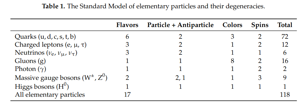
Standard model Table borrowed from arXiv:1609.04979.
For relativistic particles we have \(P_{\rm X}=\epsilon_{\rm X}/3\). From the first law of thermodynamics, if you do not have any heat transfers, then \begin{eqnarray} 0 &=& d(\epsilon_{\rm X}V) + P_{\rm X}dV\\ &=& 3d(P_{\rm X}V) + P_{\rm X}dV \\ \frac{dP_{\rm X}}{P_{\rm X}} &=& -\frac{4}{3} \frac{dV}{V} \end{eqnarray} This implies that relativistic particles behave like a gas with \(P_{\rm X}\propto V^{-4/3}\), a gas with adiabatic index \(4/3\). Using \(PV \propto T\), we obtain that the \(T\propto V^{-1/3} \propto a^{-1}\).
On the other hand, for non-relativistic particles with 3 degrees of freedom we have \(\gamma=5/3\), thus their temperature will fall as \(T\propto a^{-2}\).
Effective number of degrees of freedom for arbitrary particles:
For particles which are in between the two limits we discussed above, we have to carry out the full integrals for the number density. the pressure and the energy density. The simplest way to do these integrals is to substitute
\begin{eqnarray} {\cal E}=\frac{E}{k_{\rm B}T} \,\,\,\,\,\, {\cal M} = \frac{m_{\rm X}c^2}{kT} \end{eqnarray}
Thus,
\begin{eqnarray} n_{\rm X} &=& \int_0^{\infty} f_{\rm X} dp \\ &=& \int_0^{\infty} \frac{g_{\rm X}}{2\pi^2 \hslash^3} p^2 \left[ \exp\left( \frac{E_{\rm X}}{k_{\rm B}T}\right) \pm 1 \right]^{-1} dp \\ &=& \int_0^{\infty} \frac{g_{\rm X}}{2\pi^2 \hslash^3} p^2 \left[ \exp {\cal E} \pm 1 \right]^{-1} dp \\ &=& \frac{g_{\rm X}}{2\pi^2} \left(\frac{k_{\rm B}T}{\hslash c}\right)^3 \int_{\cal M}^{\infty} \frac{ \sqrt{{\cal E}^2-{\cal M}^2} {\cal E} d{\cal E}}{\exp {\cal E} \pm 1}\\ &=& g^{*}_{n, {\rm X}} n^{\rm rel}_{\rm B}(g=1, T) \end{eqnarray} where \begin{eqnarray} g^{*}_{n, {\rm X}} (T, M) = \frac{g_{\rm X}}{2\zeta(3)} \int_{\cal M}^{\infty} \frac{\sqrt{{\cal E}^2-{\cal M}^2}{\cal E} d{\cal E}}{\exp {\cal E} \pm 1} \end{eqnarray}
Exercise:
Show that an equivalent expression for \(g^*_{\epsilon, {\rm X}}\) is given by
\begin{eqnarray} g^{*}_{\epsilon, {\rm X}} (T, M) = \frac{15 g_{\rm X}}{\pi^4} \int_{\cal M}^{\infty} \frac{ \sqrt{{\cal E}^2-{\cal M}^2} {\cal E}^2 d{\cal E}}{\exp {\cal E} \pm 1} \end{eqnarray}
and for \(g^*_{p, {\rm X}}\) is given by
\begin{eqnarray} g^{*}_{p, {\rm X}} (T, M) = \frac{15 g_{\rm X}}{\pi^4} \int_{\cal M}^{\infty} \frac{ \left[{\cal E}^2-{\cal M}^2\right]^{3/2} d{\cal E}}{\exp {\cal E} \pm 1} \end{eqnarray}
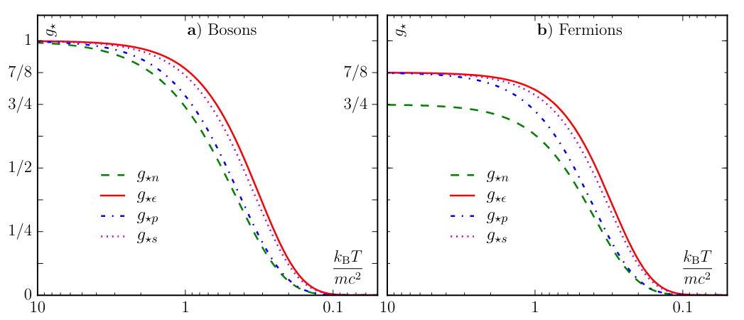
Effective degrees of freedom per intrinsic degree of freedom. Figure borrowed from arXiv:1609.04979.
For the effective degrees of freedom for entropy density of a species, note that \begin{eqnarray} s_{\rm X} &=& \frac{\epsilon_{\rm X} + p_{\rm X}}{T} \\ &=& \frac{g^{*}_{\epsilon, {\rm X}} \epsilon^{\rm rel}_{\rm B}(g=1, T) + g^{*}_{p, {\rm X}} p^{\rm rel}_{\rm B}(g=1, T)}{T}\\ &=& \frac{p^{\rm rel}_{\rm B}(g=1, T)}{T} \left[3 g^{*}_{\epsilon, {\rm X}} + g^{*}_{p, {\rm X}}\right]\\ &=& \frac{s^{\rm rel}_{\rm B}(g=1, T)}{4}\left[3 g^{*}_{\epsilon, {\rm X}} + g^{*}_{p, {\rm X}}\right] \\ \end{eqnarray} The first equality is the definition of the entropy, the second equality uses the effective degrees of freedom we calculated above for the energy density and pressure. The second equality uses \(p^{\rm rel}=\epsilon^{\rm rel}/3\). The third equality relates the pressure and entropy of relativistic particles as we had calculated before. Using the definition \begin{eqnarray} s_{\rm X} &=& g^*_{s, {\rm X}} s^{\rm rel}_{\rm B}(g=1, T) \\ \end{eqnarray} This implies that \begin{eqnarray} g^*_{s, {\rm X}} = \frac{3 g^{*}_{\epsilon, {\rm X}} + g^{*}_{p, {\rm X}}}{4} \\ \end{eqnarray}
[5]:
from scipy.integrate import quad
from scipy.special import zeta

class early_universe_particle:

    # mass_in_GeV: (m_X c^2)/GeV
    def __init__(self, mass_in_GeV, boson=True):
        self.mass_in_Gev = mass_in_GeV
        self.boson = boson
        self.zeta3 = zeta(3)

    # T_in_GeV: (k_B T)/GeV
    def effective_dof_n(self, T_in_GeV):
        curlyM = self.mass_in_Gev/T_in_GeV

        # Compute the number density effective degrees of freedom
        def dnx_integ(curlyE):
            if self.boson:
                return curlyE*np.sqrt(curlyE**2-curlyM**2)/(np.exp(curlyE)-1)
            else:
                return curlyE*np.sqrt(curlyE**2-curlyM**2)/(np.exp(curlyE)+1)

        res, err = quad(dnx_integ, curlyM, np.inf)

        return res/2./self.zeta3


    # Write code for the following functions:
    def effective_dof_eps(self, T_in_GeV):

        curlyM = self.mass_in_Gev/T_in_GeV

        # Compute the number density effective degrees of freedom
        def depsx_integ(curlyE):
            if self.boson:
                return curlyE**2*np.sqrt(curlyE**2-curlyM**2)/(np.exp(curlyE)-1)
            else:
                return curlyE**2*np.sqrt(curlyE**2-curlyM**2)/(np.exp(curlyE)+1)

        res, err = quad(depsx_integ, curlyM, np.inf)

        return 15./np.pi**4 * res

        # Write code to compute the pressure density effective degrees of freedom
        result = 0

        return result

    def effective_dof_s(self, T_in_GeV):

        # Write code to compute the entropy density effective degrees of freedom
        result = 0

        return result
[6]:
import numpy as np

boson_mass_GeV = 173.0
boson = early_universe_particle(boson_mass_GeV, boson=True)
fermion = early_universe_particle(boson_mass_GeV, boson=False)

Temperature = np.logspace(-1.0, 1.0, 50)*boson_mass_GeV
gstar_n_boson = Temperature*0.0
gstar_n_fermion = Temperature*0.0
#gstar_eps_boson = Temperature*0.0
#gstar_eps_fermion = Temperature*0.0
for ii in range(gstar_n_boson.size):
    gstar_n_boson[ii] = boson.effective_dof_n(Temperature[ii])
    gstar_n_fermion[ii] = fermion.effective_dof_n(Temperature[ii])

    #gstar_eps_boson[ii] = boson.effective_dof_eps(Temperature[ii])
    #gstar_eps_fermion[ii] = fermion.effective_dof_eps(Temperature[ii])
<ipython-input-5-6fb9b67221ab>:19: RuntimeWarning: overflow encountered in exp
  return curlyE*np.sqrt(curlyE**2-curlyM**2)/(np.exp(curlyE)-1)
<ipython-input-5-6fb9b67221ab>:21: RuntimeWarning: overflow encountered in exp
  return curlyE*np.sqrt(curlyE**2-curlyM**2)/(np.exp(curlyE)+1)
[8]:
print(boson.effective_dof_n(173.0))
print(boson.effective_dof_eps(173.0/2))
0.739577680156012
0.6579236598659057
<ipython-input-5-6fb9b67221ab>:19: RuntimeWarning: overflow encountered in exp
  return curlyE*np.sqrt(curlyE**2-curlyM**2)/(np.exp(curlyE)-1)
<ipython-input-5-6fb9b67221ab>:36: RuntimeWarning: overflow encountered in exp
  return curlyE**2*np.sqrt(curlyE**2-curlyM**2)/(np.exp(curlyE)-1)
[9]:
import pylab as pl

ax = pl.subplot(111)

ax.plot(Temperature/boson_mass_GeV, gstar_n_boson)
ax.plot(Temperature/boson_mass_GeV, gstar_n_fermion)
#ax.plot(Temperature/higgs_mass_GeV, gstar_eps_boson)
#ax.plot(Temperature/higgs_mass_GeV, gstar_eps_fermion)


ax.set_xscale("log")
#ax.set_yscale("log")
ax.set_xlabel(r"$\frac{k_{\rm B}T}{m_{\rm X}c^2}$")
ax.axhline(3./4., color="orange", linestyle="dashed")
ax.axhline(1.0, color="b", linestyle="dashed")
ax.set_xlim([10, 0.1])
[9]:
(10, 0.1)
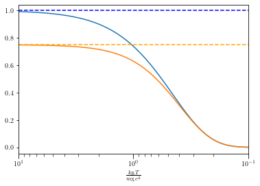
[10]:
# Now plot on log scale

ax = pl.subplot(111)

ax.plot(Temperature/boson_mass_GeV, gstar_n_boson)
ax.plot(Temperature/boson_mass_GeV, gstar_n_fermion)
#ax.plot(Temperature/higgs_mass_GeV, gstar_eps_boson)
#ax.plot(Temperature/higgs_mass_GeV, gstar_eps_fermion)


ax.set_xscale("log")
ax.set_yscale("log")
ax.set_xlabel(r"$\frac{k_{\rm B}T}{m_{\rm X}c^2}$")
ax.axhline(3./4., color="orange", linestyle="dashed")
ax.axhline(1.0, color="b", linestyle="dashed")
ax.set_xlim([10, 0.1])
[10]:
(10, 0.1)

Total effective degrees of freedom
Depending upon the temperature of the Universe we can compute the total effective degrees of freedom in all relativistic species and write down the relationship between the energy density of radiation which is driving the expansion and the temperature. For example, at very very high temperatures when all the standard model particles are relativistic, and are present in equilibrium quantities, we have 90 fermionic degrees of freedom and 28 bosonic degrees of freedom. For number densities, we have \(28 + 3/4\times 90 = 95.5\) effective degrees of freedom, for energy densities, pressures, and entropy that number is \(28 + 7/8\times 90=106.75\). That allows us to write the relations between the energy density versus temperature. As the temperature drops several particles start to annihilate, depending upon the masses of the different standard model particles. Thus their number densities will start to change as the temperature. These changes happen at specific temperatures in the Universe corresponding to the masses of the standard model particles.
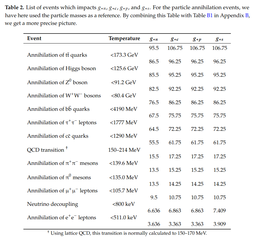
Change in the total effective degrees of freedom at different junctures. Table borrowed from arXiv:1609.04979.
Particle freeze out
If you have different species in the Universe, depending upon their masses they will go between these relativistic and non-relativistic limits. Importantly once the temperature of the Universe drops below \(m_{\rm X}c^2/k_{\rm B}\), the abundance, and the related quantities quickly undergo an exponential drop. In the radiation dominated era, the expansion of the Universe is controlled by the species that are relativistic. Once they become non-relativistic their relevance becomes less to the expansion of the Universe in the radiation dominated era. This continues until the particles remain in thermal equilibrium, and the creation and annihiliation reactions can still happen against the backdrop of an expanding Universe. Once the expansion time scale of the Universe becomes smaller compared to the annihilation rates, the abundance of particles gets frozen in, and they just fall off as \(a^{-3}\).
At early times, we can safely ignore any curvature, \(\Lambda\) and matter terms, and thus \begin{equation} \frac{\dot{a}}{a} = \left[\frac{8\pi G\rho}{3}\right]^{1/2} \end{equation} The expansion time scale is then given by \begin{equation} t_{\rm exp} = \frac{a}{\dot{a}} \propto \left[ G \rho \right]^{-1/2} \propto a^2 \end{equation} In the radiation dominated era, \(\rho \propto a^{-4}\), and thus \(t_{\rm exp}\propto a^2\). The expansion time scale thus increases rapidly.
Thermal equilibrium can be maintained mainly by two body interactions \begin{equation} \frac{dN}{dt} = n \langle \sigma v \rangle \propto n \propto T^{3} \propto a^{-3} \end{equation} The collision time scales are thus increasing as \begin{equation} \Gamma = \left[\frac{dN}{dt}\right]^{-1} \propto a^{3} \end{equation} Thus at early times the particles are in thermal equilibrium but they will quickly fall out of the equilibrium once the expansion time scale becomes shorter than the collision time scale. Depending upon when this happens the particle abundances freeze out while they are relativistic or non-relativistic. Once that happens, the energy density of matter particles just goes down as \(a^{-3}\).
Let us consider the case of neutrinos which are kept in thermal equilibrium via the weak interaction between positrons and electrons (which are in turn coupled to the photons). The interaction rate is given by (see the Particle Data group tables for \(G_{\rm weak}\),
\begin{equation} \Gamma = n_{\rm e}\sigma_{\rm weak} c \approx \left(\frac{k_{\rm B}T}{\hslash c}\right)^3 (\hslash c G_{\rm weak} k_{\rm B}T)^2 \end{equation} Here we have used the temperature dependence of the weak interactions. The Hubble expansion rate is given by the Friedmann equation \begin{equation} H = \left(\frac{8\pi G}{3c^2}\epsilon\right)^{1/2} = \left(\frac{8\pi G}{3c^2}g^*_\epsilon \frac{\pi^2}{30} \frac{(k_{\rm B}T)^4}{(\hslash c)^3}\right)^{1/2} \end{equation}
The interaction rate and the expansion rate become equal when
\begin{equation} \frac{\Gamma}{H} \approx \frac{T}{10^{10} K} \approx \frac{k_{\rm B}T}{\rm 800\, keV} \end{equation}
At these temperature neutrinos start to decouple from the rest of the electron positron photon plasma. They remain relativistic at these energies and thus their temperatures continue to drop as \(1/a\).
The radiation energy density keeps falling off as \(a^{-4}\), and thus eventually matter becomes important in driving the expansion of the Universe.
Temperature of a decoupled relativistic species
We have seen that the total entropy \(a^3s(T)\) in the Universe stays constant. However the entropy density \(s(T) \propto g^{*}_{s}T^3\). Thus we obtain that \(g^*_{s}a^3 T^3 =\) constant. When the effective degrees of freedom goes down the temperature will decrease at a slower fashion than it would normally do due to expansion.
This can be understood in the following fashion: at high temperatures particles and antiparticles annihilate and dump energy into the radiation (or lower mass particles). However the particle pair production process causes the opposite to happen and an equilibrium is maintained. However as the temperature falls, the pair production gets affected. Pair annihilations continue to dump energy in to the relativistic sector. This is the reason why the temperature drop become slower during the time when pair annihilation processes take place.
Cosmic Neutrino background
Let us consider a particle species like neutrino which decouples when it is relativistic. It happens when the temperature drops below \(800\) keV. In this case it has its own temperature (which continues to decrease as \(1/a\). This temperature is the same as the rest of the particles (electrons, positrons and photons) even after the neutrinos have decoupled (just because both the temperatures continue to fall at the same rate). However, at temperatures close to \(511\) keV, the electron-positron pair annihilations start to take place. This will cause the temperature of the photons to drop slower than the usual \(1/a\) as the electron-positron pair starts to annihilate and dump the energy in to photons. The temperature of the photons thus rises compared to that of the neutrinos.
Let us write down the temperature for photon, electron, positron plasma to be \(T_{\gamma,1}\) before the annihilation, and \(T_{\gamma, 2}\) after the annihilation. The effective degrees of freedom of the electron, positron, photon plasma before is \(g^*_{s, \gamma, 1}=2\times7/8+2\times7/8+2=5.5\). and after the annihilation is \(g^*_{s, \gamma, 2}=2\). As we discussed before \(T_{\gamma,1} = T_{\nu, 1}\). The effective degrees of freedom in neutrino sector remain the same. Let \(T_{\nu, 2}\) be the effective temperature of the neutrino species after the electron positron annihilation. The entropy conservation will imply that,
\begin{eqnarray} T_{\gamma, 1}^3 g^{*}_{s, \gamma,1}a_1^3 &=& T_{\gamma, 2}^3 g^{*}_{s, \gamma,2}a_2^3 \\ T_{\nu , 1}^3 a_1^3 &=& T_{\nu, 2}^3 a_2^3 \end{eqnarray}
Dividing one by the other we obtain
\begin{equation} T_{\gamma, 2} = T_{\nu}\left[ \frac{ g^{*}_{s, \gamma,1}}{ g^{*}_{s, \gamma,2}} \right]^{1/3} = \left[\frac{11}{4}\right]^{1/3} T_{\nu, 2} \end{equation}
Thus the temperature of the neutrino background is expected to be smaller compared to the temperature of the photon background today.
Nucleosynthesis
Next we will jump back to a time after the QCD transition phase after which the Quark gluon plasma has transformed into a hadron gas plasma. Teh quarks are now bound in neutrons and protons. And these species remain in thermal equilibrium via the weak interactions until these weak interactions freeeze out at about \(800\) keV (1 second after the big bang).
\begin{equation} n + \nu_e \leftrightarrow p + e^{-} \end{equation}
Given the masses of the neutrons and protons, they are expected to be non-relativistic at these temperatures, thus we can use the formulae for the number density of non-relativistic species to obtain
\begin{equation} \frac{n_n}{n_p} = \exp\left( -\frac{\Delta m c^2}{k_{\rm B}T} \right) \approx \frac{1}{6} \end{equation}
The mass difference \(\Delta m c^2 = 1.4\) MeV. At higher temperatures the fractions will be close to unity. However at the temperature when the weak interactions freeze out, this ratio is close to 1/6.
The neutrons and protons can also interact among themselves to form deuterium via the reaction \begin{equation} n + p \leftrightarrow \left.^2H\right. \end{equation} These reactions are again governed by the Saha equation and similar to the recombination of electrons and protons that we studied, the formation of deuterium is delayed by the high number density of photons. Instead of forming at a temperature corresponding to the binding energy of deuterium \(\approx 2\) MeV, the formation is delayed to \(\approx 80\) keV, which happens about 100s after the big bang.
During this time, the neutrons decay into protons with a half life time of 880 seconds. Thus the neutron to proton number density ratio will change further to \begin{equation} \frac{n_n}{n_p} \approx \frac{1}{6}\exp\left( - \frac{100}{886.0} \right) \approx \frac{1}{7} \end{equation} After \(80\) keV, the neutrons start to be rapidly captured by protons to form deuterium which in turn form Helium nuclei, and thus the only remaining hydorgen atoms in the Universe correspond to the protons which are not able to find the neutrons. The total mass density of the matter will then be proportional to \(n_{\rm n} + n_{\rm p}\), while the mass in hydrogen will be \(n_{\rm p} - n_{\rm n}\). The fraction of helium by mass will then be given by \begin{equation} Y_{\rm p} = 1 - X_{\rm p} = 1 - \frac{n_{\rm p} - n _{\rm n}} {n_{\rm n} + n_{\rm p}} \approx \frac{1}{4} \end{equation} where we have used \(n_{\rm n}/n_{\rm p} \approx 1/7\) in the last approximation.
The chain of fusion processes are \begin{eqnarray} n + p \leftrightarrow H^2\\ H^2 + H^2 \leftrightarrow H^3 + n\\ He^3 + H^2 \leftrightarrow He^4 + p\\ H^2 + H^2 \leftrightarrow H^3 + p\\ He^4 + H^3 \leftrightarrow Li^7 + \gamma \\ \end{eqnarray}
Detailed nuclear reaction rate tables can be used to determine the abundances of these light elements and their ratios with one another. These can then be constrained using observations.
Cosmic microwave background
As the Universe cools, electrons and protons are in equilibrium with the photon bath via the reaction
\begin{equation} e^- + p^+ \leftrightarrow H + \gamma \end{equation}
The equation which governs the number densities of the different \(H\) atom compared to the \(e^-\) and \(p^+\) is the Saha equation which describes the equilbrium number densities
\begin{equation} \frac{n_{p}n_{e}}{n_{\rm H}} = \frac{(2\pi m_{\rm e} k_{\rm B}T)^{3/2}}{h^3} \exp\left(-\frac{\chi}{k_{\rm B}T} \right) \end{equation} Here, \(\chi=(m_e + m_p - m_H)c^2 = 13.6\) eV. The total number of baryons must be conserved, thus \(n_B = n_H + n_p\), and given that we should maintain neutrality we obtain \(n_e=n_p\). Define \(x=n_e/n_B\), then \(n_H/n_B=1-x\), and we get \begin{equation} \frac{x^2}{1-x} = \frac{(2\pi m_{\rm e} k_{\rm B}T)^{3/2}}{h^3n_{\rm B}} \exp\left(-\frac{\chi}{k_{\rm B}T} \right) \end{equation} We can use \(n_{\rm B} = \eta n_{\gamma}\) to obtain \begin{eqnarray} \frac{x^2}{1-x} &=& \frac{(2\pi m_{\rm e} k_{\rm B}T)^{3/2}}{h^3n_{\gamma}\eta} \exp\left(-\frac{\chi}{k_{\rm B}T} \right) \\ &=& \frac{(2\pi m_{\rm e} k_{\rm B}T)^{3/2}}{h^3 2\frac{\zeta(3)}{\pi^2} \left(\frac{k_{\rm B}T}{\hslash c}\right)^3 \eta} \exp\left(-\frac{\chi}{k_{\rm B}T} \right) \\ &\approx& \frac{0.26}{\eta} \left(\frac{m_e c^2}{k_{\rm B}T}\right)^{3/2}\exp\left( -\frac{\chi}{k_{\rm B}T}\right) \end{eqnarray}
The value of \(\eta\) can be estimated today to be \(10^{-9}\). To obtain a value of \(x \approx 0.1\), we require \(T\sim 3000\) K. If we had naively estimated the temperature based on \(\chi=13.6\) eV, this would give a value close to \(10^5\) K instead. The reason why this recombination happens at a lower temperature is related to the small value of the baryon to photon ratio.
Until the Universe remains ionised, the photon free path is very small. Once the photon temperature drops to \(T<3500\) K, the photons are no longer energetic enough to ionise the hydrogen atoms, and they start to free stream. These photons that started free streaming after the recombination of the electrons with the protons can be observed today in the microwave at a temperature of \(T=2.726\) K. This is the cosmic microwave background radiation.
Cosmological parameters from the cosmic microwave background
The cosmic microwave background was discovered by Arnos Penzias and Robert Wilson in 1965, work for which they received the Nobel Prize in Physics. This is a remarkable achievement, the existence of this relic radiation from the Universe’s hot past was predicted by Gamow and colleagues even before it was observed (there was a large uncertainty about the exact temperature though). There was a huge experimental effort to detect fluctuations in the CMB, but to no avail. Without fluctuations you cannot form all the structure that we see in the Universe today. This non-existence of detectable fluctuations remained a conundrum for a few decades before observational progress made it possible to observe the fluctuations.
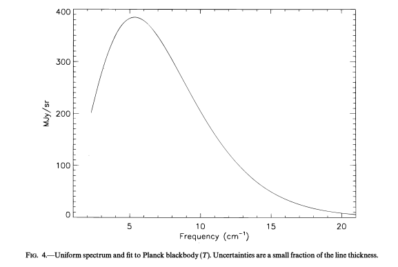
The energy spectrum of the cosmic microwave background radiation was measured by the COBE satellite in 1990s. The spectrum is shown below along with a fit to a black body spectrum. The figure does not have any visible errorbars because the errors are smaller than the thickness of the line!
Armed with these measurements, the COBe team was able to make a detailed map of the fluctuations in the cosmic microwave background. The figure below shows the temperature measurement in the top plot as a function of position on the sky, the middle panel shows the residual after removing the monopole component, and shows the dominant dipole fluctuation due to the motion of galaxy with respect to the CMB frame/ The bottom panel shows the residual fluctuations after both the monopole and dipole are subtracted out.
First notice the degree to which the CMB is isotropic, the temperature scale is in Kelvin in the top panel, millikelvin in the middle panel and microkelvin in the bottom. The CMB fluctuations are extremely tiny of the order \(10^{-5}\) of the monopole. These fluctuations are our earliest look at the fluctuations which caused the formation of structure in the Universe.
These fluctuations tell us a lot of information about the Universe. We will make an attempt to understand the most basic information given by the fluctuations of the CMB. As we have seen before, the CMB is relic radiation belonging to an era when the baryons and photons were tightly coupled with each other. As the temperature dropped the electrons could no longer be ionized from hydrogen atoms, and the photons started to stream freely.
Let us try to understand how big would be the typical size of a fluctuation in the CMB. To understand this we need to understand how fluctuations behave in the baryon photon plasma. Recall that the pressure and density of relativistic photons are related as \(p = \rho c^2/3\). Thus the speed of any pressure density fluctuations in photons and any matter coupled with radiation will be close to \(c_{\rm s}^2 = dp/d\rho \approx c/3\). There are small corrections to this equation due to the non-zero fraction of baryon to photon energy density, but let us neglect it for the moment. Any pressure-density perturbations in the plasma will propagate with the sound speed in the plasma. These fluctuations will begin to travel from the moment they were created to the moment the baryons lose their coupling with the photons (which happens at recombination).
Exercise:
Use \(\Omega_{\rm m}=0.3\) and \(\Omega_{\rm r}=8\times 10^{-5}\) to figure out the scale factor of the epoch at matter radiation equality. Compute the temperature of the Universe at the epoch of matter radiation equality if the temperature of the Universe today is \(2.726 K\). Compare this temperature to the temperature at which CMB is released.
If we have a drum and we excite it with different frequencies we can see different modes of the fluctuations of the surface of a drum:
[6]:
YouTubeVideo("v4ELxKKT5Rw", width=800)
[6]:
When you beat a drum you excite all these different modes.
Similarly density perturbations travel in the early Universe and we can carry out a fluctuation analysis in terms of the modes. These modes are observed as projected on to the sky. We can compute the two point correlation function of the temperature fluctuations in the CMB as a function of separation between these scales \(\theta\). Consider two direction \(\hat{n}\) and \(\hat{n}'\) with \(\hat{n}.\hat{n}' = \cos\theta\). Then we can compute \begin{equation} C(\theta) = \langle \Delta T(\hat{n}) \Delta T(\hat{n}') \rangle_{\hat{n}.\hat{n}' = \cos\theta} \end{equation} This correlation function can be decomposed in to modes by taking a spherical harmonic transform (this is like an angular decomposition of modes rather than a Fourier decomposition) to obtain the power spectrum \(C_{\rm l}\). \begin{equation} C(\theta) = \sum_l \frac{2l+1}{4\pi} C_l P_l \cos(\theta) \end{equation} Each Legenedre polynomial is an oscillating function where the oscillation increase as \(l\) increases. The characteristic scale of each oscillation is inversely proportional to \(l\). The temperature fluctuation power spectrum looks like the one shown below:
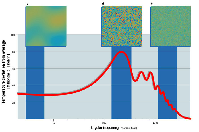
Figure borrowed from Hu and White (Sci Am 290N2 44 (2004) ).
We can see that we have power at different angular frequencies in the CMB power spectrum, we can detect a clear first peak, and then a series of overtones.
The first peak corresponds to the fundamental mode where fluctuations start at the maximum at the beginning of the Universe and reach the minimum at decoupling (or vice versa). The wavelength of this mode will equal the distance sound waves can travel from the beginning of time to the epoch of decoupling. We know the speed of sound in the baryon photon plasma and we can use this to compute the sound horizon at recombination.
\begin{equation} r_{\rm s}^* \approx \int_{0}^{t_{\rm rec}} \frac{c}{\sqrt{3}} dt \end{equation}
We can change variables to the scale factor \(a\) with the help of the Friedmann equation. Remember a large fraction of the time between the beginning of the Universe and the decoupling will be dominated by the matter dominated epoch. Thus we can use the simplified Friedmann equation to compute the sound horizon at recombination \begin{eqnarray} r_s^{*} &\approx& \frac{c}{\sqrt{3}} \int_{0}^{a_*} \frac{a}{\dot{a}} \frac{da}{a} \\ &=& \frac{c}{H_0\sqrt{3\Omega_{\rm m}}} \int_{0}^{a_*} a^{1/2} da \\ &=& \frac{2c}{3H_0\sqrt{3\Omega_{\rm m}}} a^{3/2} \end{eqnarray}
This is a physical scale in the Universe, we observe the fundamental mode at a particular angular scale when we measure the temperature fluctuations. The two are related by the angular diameter distance, computed between us and the surface of last scattering. This angular diameter distance is dependent on the cosmological constituents of the Universe which dominate the energy density budget of the Universe after recombination. These will thus include the matter density parameter, curvature and the dark energy density. Thus the angle
\begin{equation} \theta_s^* = \frac{r_s^*}{D_{\rm ang}(a_*)} \end{equation}
is a physical observable which depends on the cosmological parameters. And we can use the measurements to constrain cosmological parameters. It can be shown that the primary sensitivity of this angle \(\theta_*\) is to the curvature of the Universe. In particular, by varying cosmological parameters one can show that \begin{equation} l_{\rm first peak} \approx \frac{200}{\sqrt{1-\Omega_{\rm k}}} \end{equation}
These peaks have been measured pretty precisely now. The first peak is at degree scales, and is the biggest hint that the Universe is very close to having a flat geometry.
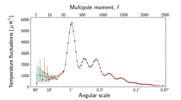
Figure borrowed from the Planck website, please take a look at the URL of the image for reference.
The relative height of the second peak compared to the first tells us about the baryon density of the Universe, while the relative height of the third peak tells us about the dark matter density in the Universe, a mysterious component of the Universe which we understand very little about. Given the accuracy with which the peaks have been measured, the cosmic microwave background helps us understand the constituents of the early Universe with very high precision and accuracy.
Figure borrowed from the Planck collaboration
Exercise:
Show that the ratio of the energy density of photons to that of neutrinos at decoupling is \(\approx 1.5\). You can use that the temperature of the neutrinos compared to the temperature of photons is \([4/11]^{1/3}\) as derived earlier. Use the number of degrees of freedom for each species, and the expressions of energy density for relativistic particles.
Reference material for reading about the cosmic microwave background:
Excellent material can be found on Wayne Hu’s CMB tutorial page: Beginner level introduction followed by Intermediate level and a review article in Scientific American .
\begin{equation} \frac{dP_{\rm X}}{dT} = \frac{P_{\rm X}+\epsilon_{\rm X}}{T} \end{equation} First differentiate the pressure expression with respect to \(T\), change the variable from \(p\) to \(E\) and then integrate the expression by parts using the formula \begin{equation} \int u v dw = uvw - \int u w dv - \int v w du \end{equation} Then use this in combination with \begin{equation} \frac{d}{dt}\left[ a^3 \rho c^2 \right] + p \frac{d}{dt}\left[ a^3 \right] = 0 \end{equation} to show that the entropy density of the Universe is conserved. \begin{equation} \frac{d}{dt}(a^3 s) = 0 \end{equation}
\begin{equation} T= 1\,\text{MeV}\, \left[\frac{t}{1 s}\right]^{-\frac{1}{2}} \end{equation}